Libra: An open-source "Methodology Discovery" Library

Classical Molecular Dynamics Tutorial

This tutorial shows how to run classical molecular dynamics (MD) simulations of atomistic systems under various conditions. In principle, you can use these examples as a template for your particular calculations (also meaning you'd need to modify only very few parameters). The working files showing how to use different objects are located in the /tests/test_md directory of the Libra package.

Before doing this tutorial, it is recommended to go through the Molecular Mechanics tutorial, because it explains the main components and the operations (the creation of molecular system, force fields, hamiltonians, setting up interactions, organizing MD workflow) of the run_aa_md_state.py file. This is the file we are to run in each sub-directory of the present tutorial. It is almost the same for all cases, except for few places in which we introduce certain variations.

This is the first example in this tutorial, so we'll discuss some common elements here. In the later examples, we will focus only on the distinctions between the cases.

The initial workflow for initialization is the following:

• Unitialize random number generator, create a Universe object and load data into it, create force field object and load data:

  rnd = Random()
  U = Universe(); LoadPT.Load_PT(U, os.getcwd()+"/elements.txt")
  uff = ForceField(...)
  LoadUFF.Load_UFF(uff,"uff.dat")
  

• Create molecular structure by loading a molecule from a file, initialize internal variables

  syst = System()
  LoadMolecule.Load_Molecule(U, syst, "Pc-C60.ent", "pdb")
  syst.determine_functional_groups(0)  # do not assign rings
  syst.init_fragments()
  

• Create an atomistic (MM type) Hamiltonian, perform initialization of internal variables (interactions), bind the Hamiltonian to the molecular system of interest (so that the energy/force evaluation is sensitive to the changes of the molecular structure "syst"), and perform the first energy/force evaluation

  ham = Hamiltonian_Atomistic(1, 3*syst.Number_of_atoms)
  ham.set_Hamiltonian_type("MM")
  ham.set_interactions_for_atoms(syst, atlst1, atlst1, uff, 1, 0)  # 0 - verb, 0 - assign_rings
  ham.set_system(syst);   ham.compute()
  

• Initialize some dynamic variables (not really used in these simulations, but are needed for other procedures)

  el = Electronic(1,0)
  mol = Nuclear(3*syst.Number_of_atoms)
  nve_md.nve_md_init(syst, mol, el, ham)
  

So far we have performed only the initialization. Now, we can proceed to actual dynamics. In fact, the rest of the script does two types of dynamics: cooling (optimization by a simulated annealing) and the production MD. In addition to the previous tutorials, we now utilize the State class of the libscript library. The State class is designed to represent a thermodynamic state of the system. That is it encodes the state (coordinates/velocities) of the system, as well as the state of the bath (thermostat/barostat). It also contains information about the macroscopic and miscroscopic observables: potential, kinetic, total energies, extended system-bath energy, current temperature, pressure, simulation cell shape and volume, and other variables.

Together with the State class, we use an auxiliary MD class, defined in the same header. This class is essentially a container for the MD settings. So, we first create an object of MD type and then pass it to the State object to tell it how to perform MD simulations:

md = MD({"max_step":1,"ensemble":"NVE","integrator":"DLML","terec_exp_size":10,"dt":20.0,"n_medium":1,"n_fast":1,"n_outer":1})

Here, we utilize a constructor that takes a Python dictionary and extracts values for the keywords relevant to/defined in the MD class.

The State class has several methods for setups, initialization, and actual simulations. Lets look closely at some of them:

• ST.set_system(syst)- Bind the System type object to the State type object, so that all changes made to the "syst" variable are known to the "ST" object, and vice versa - all changes made internally by the "ST" object are reflected in the variables of the "syst" oobject.
• ST.set_md(md) - Bind the external md object to the ST object. So, once this is done, we can change the internal MD settings of the ST object by changing the corresponding variables of the external md object. For instance, this can be used if we run several rounds of MD or optimization. In the first rounds of optimization, we may want to use smaller MD integration timesteps md.dt, so do not destroy the system. On the later rounds, we can increase this value (up to the stable integration limit), so to accelerate the convergence. We can also vary the number of the MD steps performed in a sinle call of the "run_md" funciton (see below). This number is accessed by md.max_step. Again, if you do an optimization, you may want to start with this number being relatively small (1 - 10). As you acheive the equilibrated state, you may icrease it. This parameter can be used to control/design the simulated annealing protocols. Finally, what you may want to change in md between one run to another, is the ensemble type: you can start with the NVT and then switch to NVE. This is accessed by the md.ensemble variable. Note, that to run an NVT simulation, you'd need to bind a thermostat to the ST object. So, generally it is easier to switch from NVT to NVE (still keeping the thermostat) than from NVE to NVT (would need to bind a thermostat, and reinitialize some internal variables, which may be not totally exact what you want to do).
• ST.init_md(mol, el, ham, rnd) - This function simply runs the consistency/sanity check and initializes all needed variables. The function must be called prior to "run_md".
• ST.run_md(mol, el, ham) This function runs an MD simulation on the system bound to the ST object as described by the md object also bound to the ST object. Note: this is not a single MD step - rather it may be many steps. This function also propagates states of thermostat or barostat objects coupled to the ST object.
• ST.cool() This function "cools" the system and thermostat by setting all atomic momenta/velocities to zero and by resetting thermostat variables to a lower-energy state (so that they could absorb more energy). Together with "run_md" constitutes a simulated annealing procedure.

The current micro/macroscopic descriptors of the State can be accessed via the exported variables:

• ST.E_kin kinetic energy of the system
• ST.E_pot potential energy of the system
• ST.E_tot total energy of the system
• ST.H_NP the extended system energy (Nose-Poicare Hamiltonian, or a Nose-Hoover invariant)
• ST.curr_T current kinetic energy of the system
• ST.curr_V current volume of the simulation cell
• ST.curr_P current pressure of the system

Please see the header file or a corresponding section of the Documentation, for a more comprehensive list of variables

To summarize, the workflow of the simulation part is following:

• Create control variables: MD, thermostat, or barostats (if needed)

  md = MD({"max_step":1,"ensemble":"NVE","integrator":"DLML","terec_exp_size":10,"dt":20.0,"n_medium":1,"n_fast":1,"n_outer":1}) 
  therm = Thermostat({"Temperature":278.0,"Q":100.0,"thermostat_type":"Nose-Hoover","nu_therm":0.01,"NHC_size":5})
  

• Create a State object and bind system, thermostat (for NVT or NPT) or barostate (for NPT or NPH) to it, setup MD control:

  ST = State() 
  ST.set_system(syst);
  #    ST.set_thermostat(therm)
  ST.set_md(md)
  

• Initialize (internal) State variables:

  ST.init_md(mol, el, ham, rnd)
  

• Run several cooling cycles

  for i in xrange(...):
      ST.run_md(mol, el, ham)        
      ST.cool()
  

• Run the MD production

  for i in xrange(...):
      ST.run_md(mol, el, ham)        
  

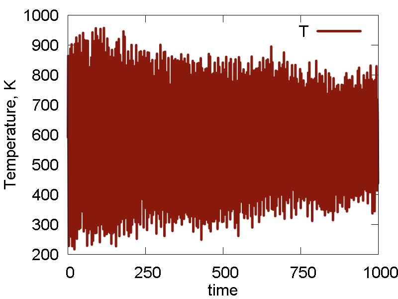
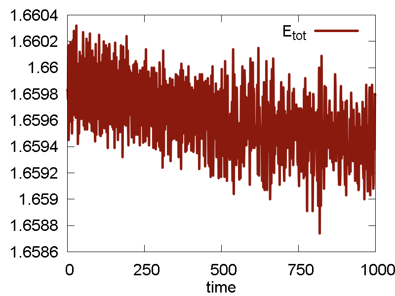
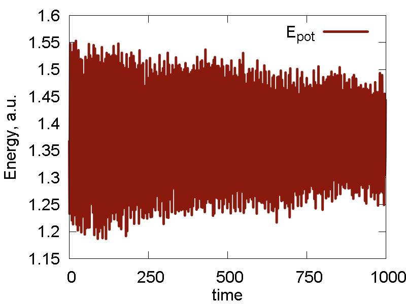
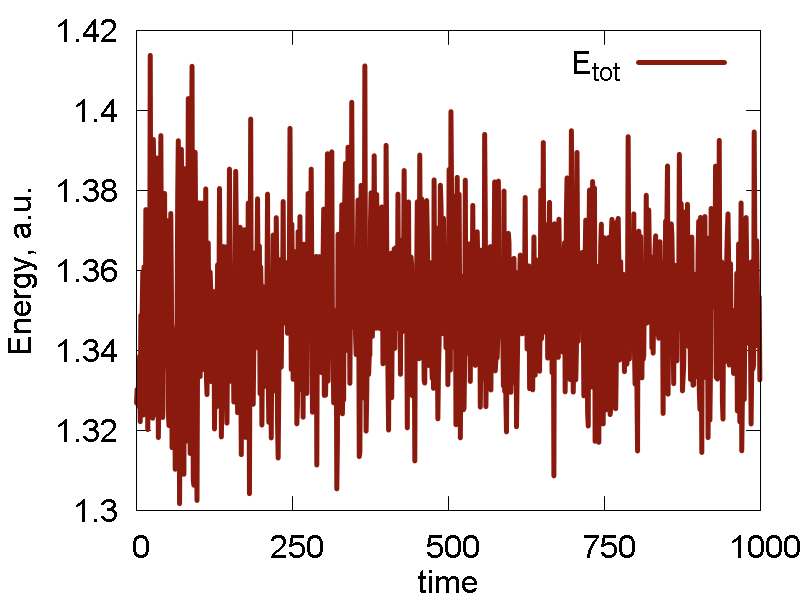
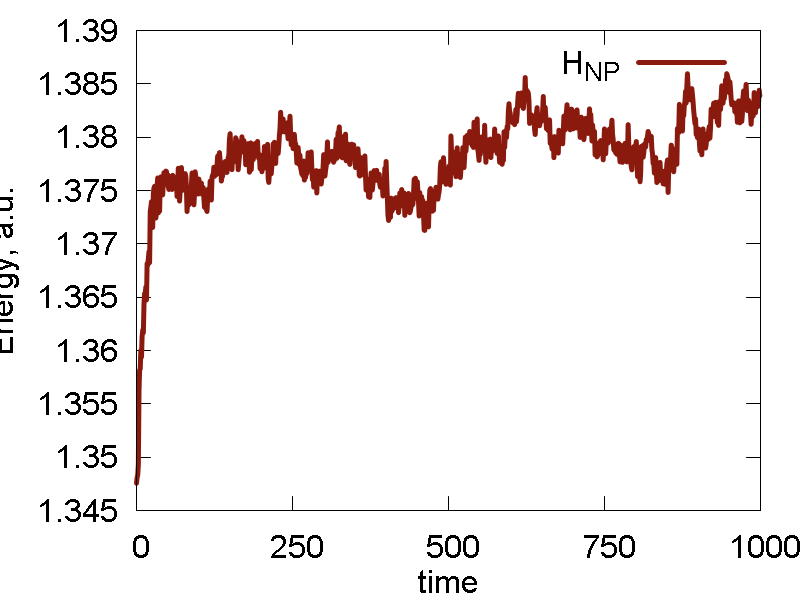
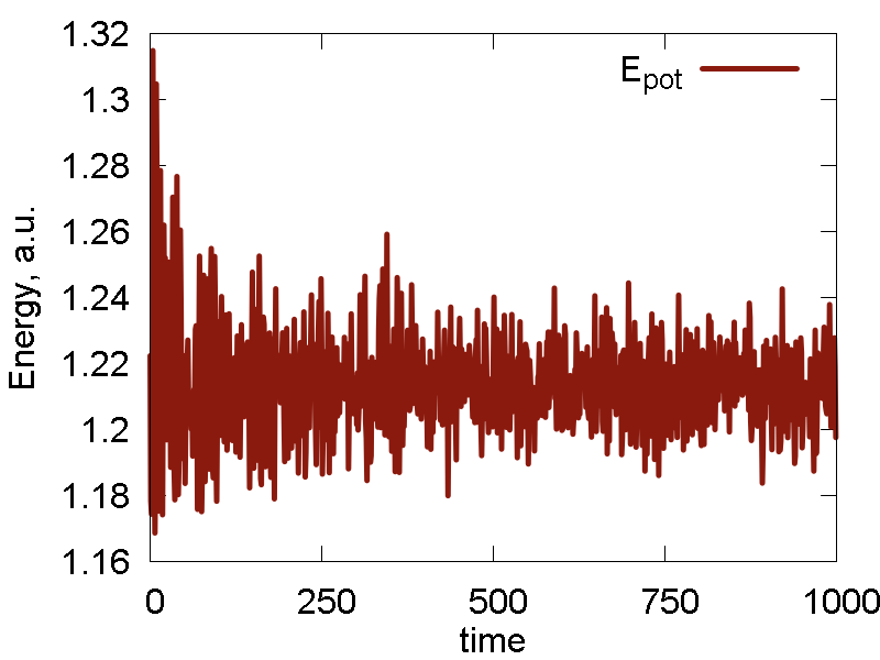
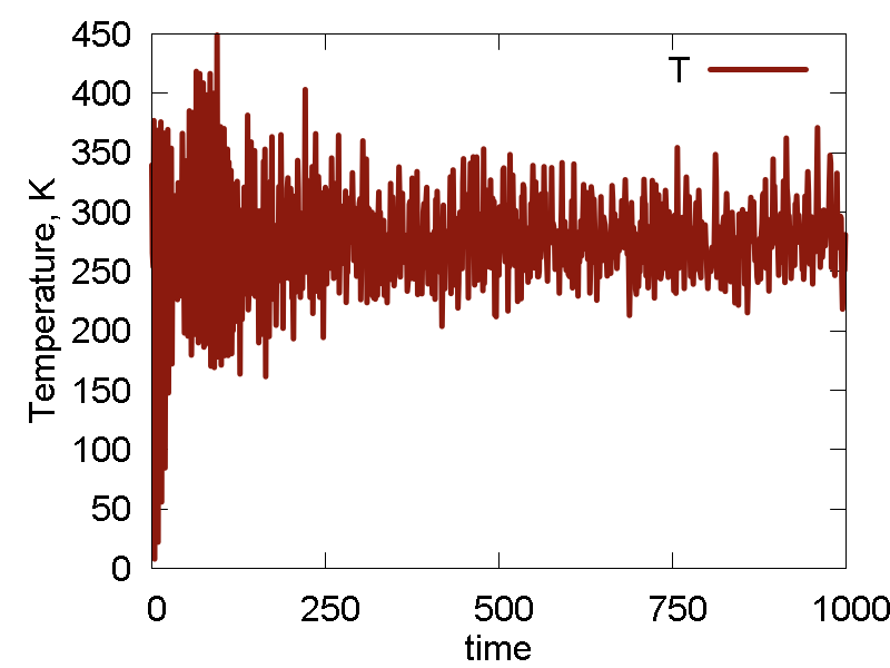
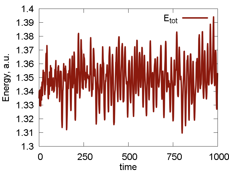
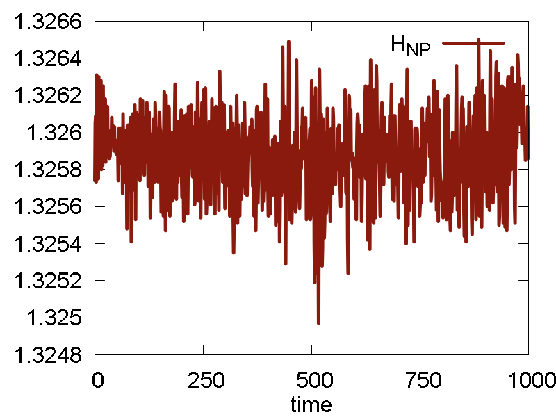
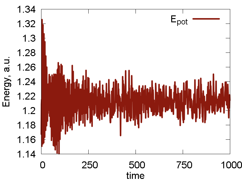
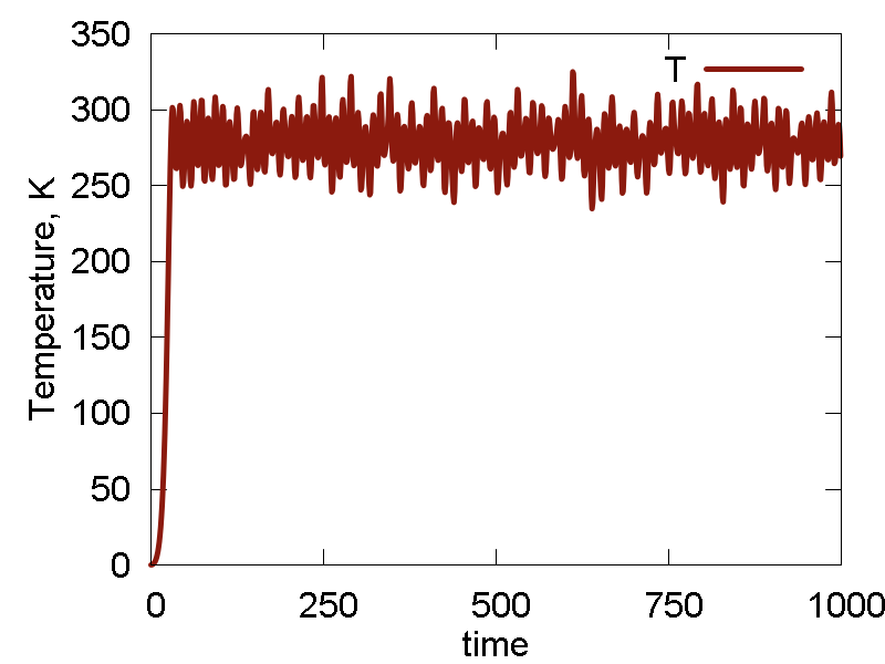
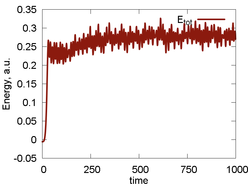
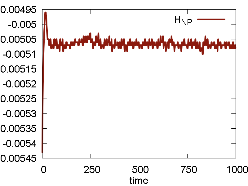
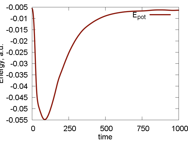
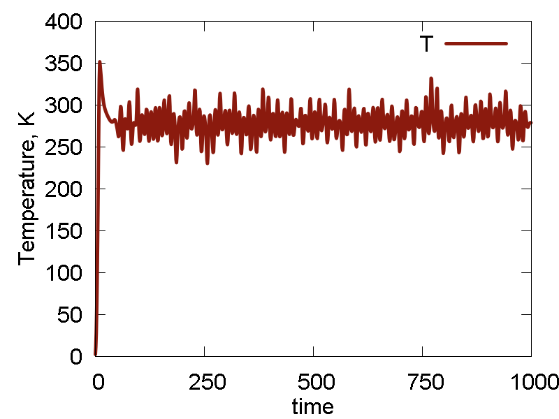
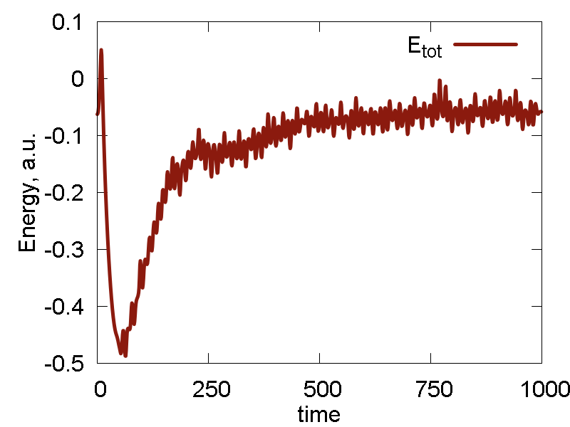
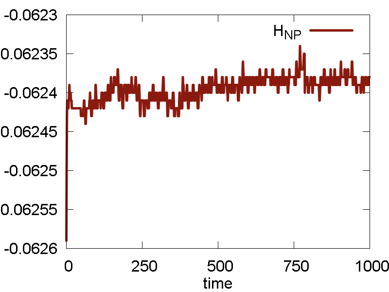
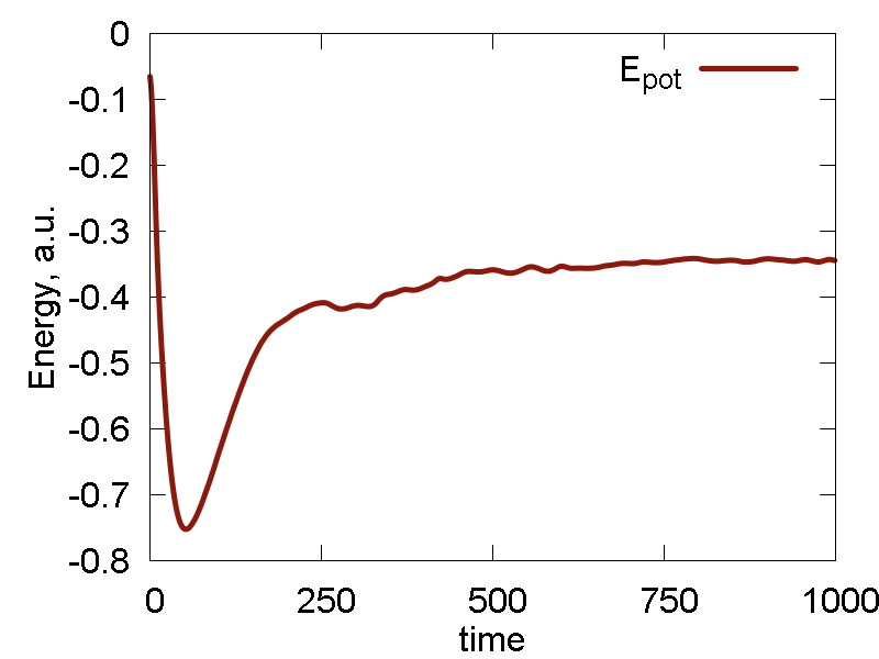
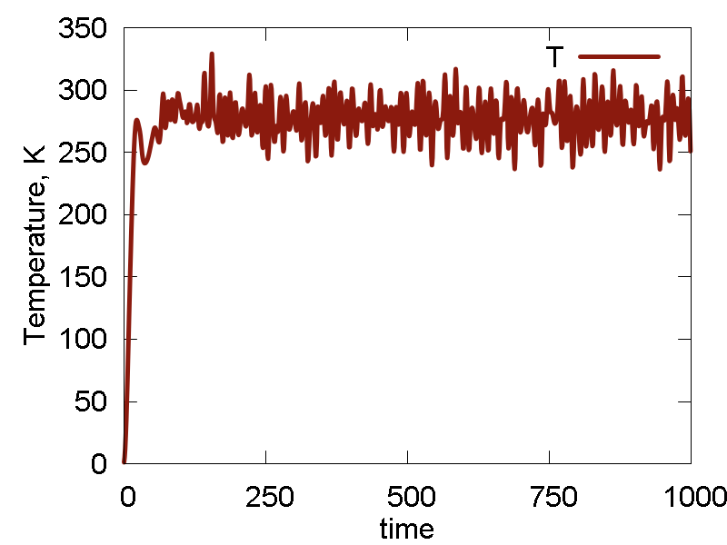
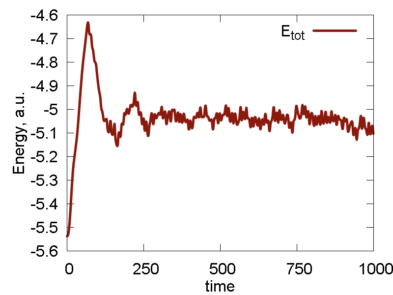
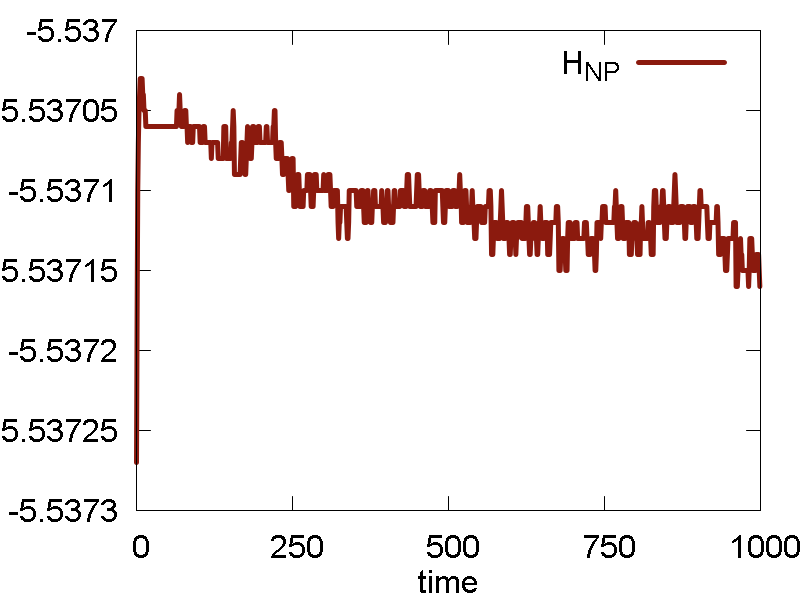
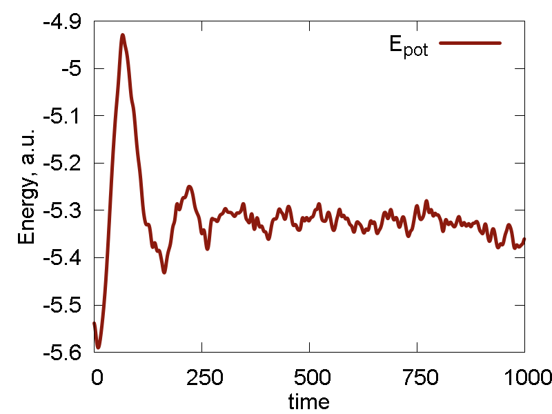
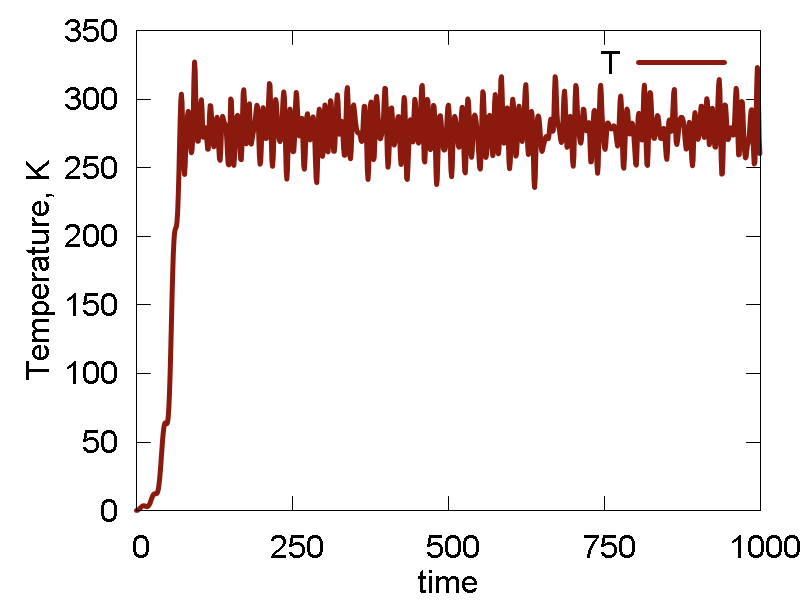
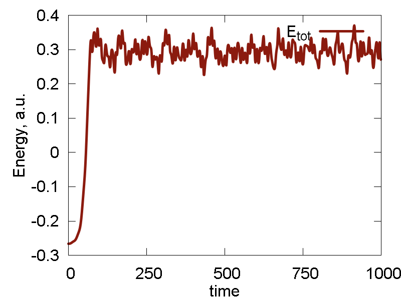
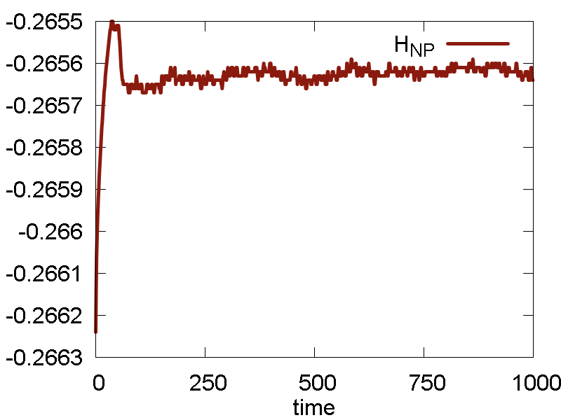
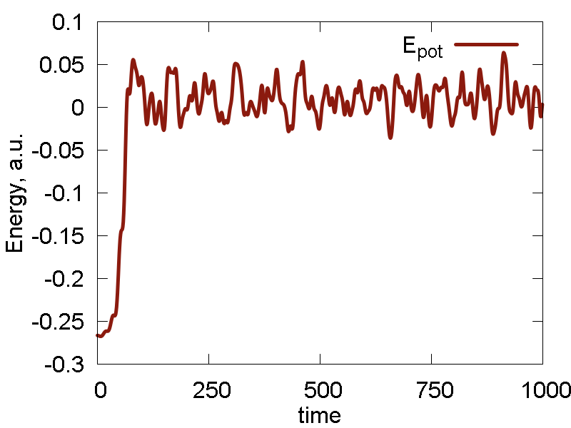
To analyze the MD run and to assess its quality, we plot some of the obervables in Fig. 1. We also show a video of the MD simulation (10 ps).

What we see:

• The dynamics is rather erratic, intermolecular separation fluctuates a lot. Temperature fluctuates a lot. Total energy and the conserved quantity show small decay (deviation from a straight horizontal line). These effects are largely due to the lack of equilibration and the choice of the initial configuration away from the energy minimum. Thus, the potential energy converts to the kinetic, so we see a lot of temperature fluctuations, and hence the molecule shows very erratic motion. The lack of initial thermalization also contributes to the deviation of the total energy/conserved quantity from the horizontal line, due to larger numerical errors in the beginning.
• The conserved quantity is the same a the total energy. This is true for NVE ensembles, or for NVT or NPT when thermostat/barostat inertia parameters ("masses") are very large.
• Potential energy fluctuation is much larger than the total energy/conserved invariant fluctuation. This means the integration scheme and parameters are reasonable.

We extend the previous case by actually adding a thermosat:

therm = Thermostat({"Temperature":278.0,"Q":100.0,"thermostat_type":"Nose-Hoover","nu_therm":0.01,"NHC_size":5})
ST.set_thermostat(therm)

and by setting the "md.ensemble" variable to "NVT":

md = MD({"max_step":100,"ensemble":"NVT","integrator":"DLML","terec_exp_size":10,"dt":20.0,"n_medium":1,"n_fast":1,"n_outer":1})

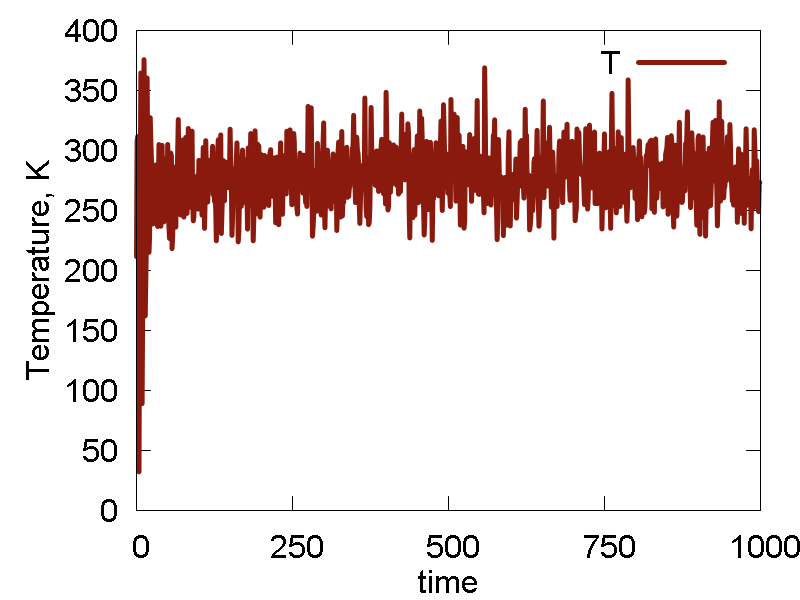
We also do several cycles of cooling, before the NVT simulation. The results are shown in Fig. 2

What we see:

• The nuclear dynamics is more regular: geometry stays more-or-less fixed, with typical high-frequency stretching modes. Relative reorientation of the two molecules is observed at a longer timescale. The intermolecular distance fluctuates only little. Temperature fluctuation is much smaller than before, with the mean corresponding to the thermostat parameters. All these effects are due to proper prior thermalization and the presence of thermostat with reasonable parameters.
• The conserved invariant is now different from the total energy (kinetic + potential) of the system. Here, the total energy shows large fluctuations, comparable to those of the potential energy. The conserved property show much smaller fluctuations. The conserved property don't show much of drift (at list on this timescale), meaning it is reasonably accurate for the present purpose. A typical "saturation" (sigmoidal) curve is observed in H_NP vs t. This is due to initial equilibration between system and thermostat (bath). This is normal, but the initial equilibration period may be not suitable for the calculations of some properties (due to its nonequilibrium nature)

Everything is same as in the previous case (case 2). The only difference is that we decrease the frequency of the thermosat (increase inertia):

therm = Thermostat({"Temperature":278.0,"Q":100.0,"thermostat_type":"Nose-Hoover","nu_therm":0.001,"NHC_size":5})

The results are shown in Fig. 3

What we see:

• The nuclear dynamics remains similar to that in the previous case.
• The conserved invariant is conserved much better: the magnitude of fluctuations decreases, the overall drift decreases (this may be especially important for longer simulations), no equilibration period observed (no "saturation", just a horizontal line).

Now, lets consider a different type of systems. Instead of organic, go to inorganic. So, try gold. This is a bigger crystal created with a script (see another tutorial) that generates a supercell good for modeling systems with Au(111) surface. Instead of molecular, go to crystalline. Well, we start with periodic-looking structure, but since there are no actual periodic boundary conditions applyed, the system is still a formally molecular one (isolated cluster).

Because this particular system consists of atoms, rather than molecules, there are no bonded interactions (bond stretching, angle bending, dihedrals, imporopers, etc). Moreover, the system is not charged, so there are no electrostatic interactions either. The only type of interactions remaining are the vdw interactions. So, the setup of the ForceField object can be simplified:

uff = ForceField({"mb_functional":"LJ_Coulomb","R_vdw_on":40.0,"R_vdw_off":55.0 })

The second important alteration made in comparison to the Example 1 scripts, is that the format of the input file defining molecular structure is different from the one we used before. The present file format follows closely the official pdb format. That is why we load it using the option "true_pdb" in the Load_Molecule function:

LoadMolecule.Load_Molecule(U, syst, "au.pdb", "true_pdb")

We start simulating the Au cluster using the default UFF Lennard-Jones (LJ) parameters for Au atom: `epsilon = 0.039` and `sigma = 3.293`. The results are shown in Fig. 4

What we see:

• The system dissociates: interatomic interactions are too weak to resist thermal activation, to the overall cluster simply evaporates/sublimates
• As the system exands to the infinity, it passes the configuration that delivers a minimum (at least along this direction) of the potential energy, with the minimal value of ca. -0.055 a.u. The following expansion brings the system to the state with potential energy approaching zero. That state corresponds to infinite separation of all Au atoms from each other (and hence Au-Au interaction approaches zero). In a sense, the dynamics scans (only by chance) the potential energy surface along the "crystal" expansion coordinate.
• As the minimal value of the potential energy is on the order of 0.055 a.u., the total energy turns out to be on the order of 0.3 a.u., implying the kinetic energy is much larger than the interatomic interaction energy. It then clear why the system sublimates.
• Temperature fluctuates around the specified value. The invariant quantity fluctuates only little. The magnitude of such fluctuation is much smaller than the total energy fluctuation. So, the integration and thermalization is going on well.

Ok. We now run one more simulation with the `epsilon` parameter of Au scaled by the factor of 10: `epsilon = 0.39`. The results are shown in Fig. 5

What we see:

• Temperature and invariant fluctuations - all is fine.
• Potential energy approaches some negative value. Also, the total energy approaches somewhat negative value (although not far from 0.0). These plots suggest that the system does not dissociate fully - some atoms will stay bound.
• Incomplete dissociation: this prediction is also supported by the visualization of the dynamics. We can see how the Au cluster sublimates, but smaller clusters are also forming.

Lets keep the parameters changing even more. We now set `epsilon = 2.8` and reduce `sigma` to `sigma = 3.0` (well, we could be just with the `epsilon` parameter alone, but I was curious to try a new thing). The results are shown in Fig. 6

What we see:

• Temperature and invariant fluctuations - all is fine.
• Both potential and total energies are sufficiently negative for the whole duration of time. No relaxation dynamics is observed except for a very short time, meaning the parameters lead to a reasonably stable system.
• From the MD visualisation, we observe pretty stable lattice dynamics. It can well correspond to a heated metal, although a bit stronger interactions may be more accurate.

So, we know how to produce a stable Au cluster in isolated molecule calculations. Now, it is time to switch to a bit more complex case - periodic systems. We will not run an MD with periodic boundary conditions (PBC), which means the atoms are always confined into the simulation box and they interact with their own replicas (and replicas of all other atoms) in the periodically translated nearby boxes.

We start with the scripts and parameters from the case 2: `epsilon = 0.39` and `sigma = 3.293`. On top of that we introduce two additions:

• We define a simulation box, via the properties of the syst object:

  T1 =  VECTOR(32.6970772436, 0.0, 0.0)
  T2 =  VECTOR(16.3485386218, 28.3164995224, 0.0)
  T3 =  VECTOR(0.0, 0.0, 26.6970517757)
  syst.init_box(T1, T2, T3)
  

  This is sufficient to tell the State functions that the simulations are for a periodic system.
• Previously, we utilized an "LJ_Coulomb" functional for vdw interactions. At this point, it is good only for the isolated systems. It would not work when a periodic box is defined. So, we choose an appropriate functional that incorporates periodic effects:

  uff = ForceField({"R_vdw_on":10.0,"R_vdw_off":12.0, "mb_functional":"vdw_LJ1","mb_excl_functional":"vdw_LJ1"})
  

Everything else remains as before. The simulation results are summarized in Fig. 7

What we see:

• Temperature and invariant fluctuations - all is fine.
• In the MD visualization, we see that the system remains crystalline. Hops of the surface atoms from one surface to the opposite one are observed (due to PBC). The internal atoms show some lattice vibrations. Although the system remains confined, it is not a solid. Rather, it is a partially melted one (remember, the system would dissociate to smaller clusters if not the periodic box).
• Potential energy is close to zero. The total energy is large positive number. This suggests the system behaves as a gas (even not as the partially melted solid).