Molecular Mechanics and Molecular Dynamics Tutorial
The "libhamiltonian_mm" is a module that implements molecular mechanics (MM) methods for computing interactions in atomistic systems. The working files showing how to use different objects are located in the /tests/test_hamiltonian_mm directory of the Libra package. Most of the tutorials are almost completely self-explanatory. Here, we only focus on most interesting/less straightforward conventions and articulate some of our actions.
test_mm1.py
We are now ready to study our first tutorial. This tutorial doesn't print much of fancy output, nor it does some complex calculations. Rather, this script demonstrates the basis steps of how to create the objects of main data types we would need for atomistic simulations.
- First, we load the auxiliary modules that implement methods for reading parameter and input files.
from LoadPT import * # Load_PT
from LoadMolecule import * # Load_Molecule
from LoadUFF import*
- Second, we create the "Universe" object and setup some properties of our Universe:
# Create Universe and populate it
U = Universe()
verbose = 0
Load_PT(U, "elements.dat", verbose)
Here, "Load_PT" is the function that is defined in the LoadPT module. It populates the object "U" using the properties defined in the file "elements.dat". The verbosity of the operations is controlled by the flag "verbose"
- To create an atomic system from a given file, we use
#======= System ==============
syst = System()
Load_Molecule(U, syst, os.getcwd()+"/Clusters/2benz.ent", "pdb")
The "Universe" object "U" is needed. In this example, the file to be loaded is located in the "/Clusters" directory and is called "2benz.ent". This is the pdb-type format with some modifications. In particular, the last column of each "HETATM" record is considered to contain the partial charge of the atom. To understad wich other options are available and which formats correspond to them, look into the LoadMolecule.py file. Alternatively, you can define your own format to read and the way to handle that format. - One can ask Libra to automatically determine the functional groups (for organic molecules) this is done via:
syst.determine_functional_groups(0) #
The parameter of the function controls whether the ring-determination procedure should be used (1) or not(0). Knowledge of the rings is needed for the correct assignment of MM atomic types, although often the differences are negligible and one may skip rign-determination option. For UFF, for instance, this would mean the sp2-hybridized C atoms would be assigned to types "C_2" rather than "C_R". The reason why one would want to skip the rign-determination step is because it may be rather time-consuming (for very complex structures) and is not perfect yet. For the full list of possible functional group names and the way the determination procedure works, refer to the file System_methods4.cpp. - Once the system is created and functional groups are determined (optionally), we can print some information about the system, to find out
whether the system is what we expect.
sys.show_atoms()
syst.show_fragments()
syst.show_molecules()
Note that when the overall system is loaded, we determine not only the bonds, angles, dihedrals and so, but also the partition of the overall system into molecules. Each disconnected from all other sub-graph of the graph of the entire system defines a molecule. So, in our case, we have loaded 2 benzene molecules. And this information is confimed by the output of the "show_molecules()" function. In our "2benz.ent" file have also provided definition of the rigid fragments (not the same as functional groups): each molecule is treated as rigid fragment. By default, if no definition of fragments is provided explicitly, each atom is treated as a separate fragment. - In the next step, we create an empty "ForceField" object named "uff" (you could choose any other name, of course, it is just convenient).
We then load the UFF parameters and settings into this object from the file, using the "Load_UFF" function of the LoadUFF.py module.
#======= Parameters ==============
# Create force field objects
uff = ForceField()
# Load parameters
Load_UFF(uff)
- So far, we have loaded only the parameters. However, any force field is a combination of the parameters set and the choice of appropriate
functional. So, we need to define the functionals for computing interatoric energies.
# Set up functional forms
uff.set_functionals({"bond":"Harmonic","angle":"Harmonic","vdw":"LJ12_6"})
The "set_functionals" method takes a dictionary argument that contains pairs of type: "potential-type":"choice of the potential of given type". The full list of possible options can be found in the "set_interaction_type_and_functional" function in the Hamiltonian_MM_methods1.cpp.
test_mm2.py
As usual, we started with the test_mm1.py script and added new features to show.
-
One of such features is the initialization of atomistic Hamiltonian - not just any atomistic one, but the one which relies on molecular mechanics (MM). This is done via:
ham = Hamiltonian_Atomistic(1, 3*syst.Number_of_atoms)
ham.set_Hamiltonian_type("MM")
However, the above instructions only create a default Hamiltonian object "ham" and set its internal properties (Hamiltonian type) to be molecular mechanics. No actual way of computing interactions is created yet. Before we can start actual computations, we need to setup interactions within this Hamiltonian. This is done via the function "set_interactions_for_atoms":
ham.set_interactions_for_atoms(syst, atlst1, atlst1, uff, verb, assign_rings)
Most of the arguments of the function are relatively straighforward to understand. Perhaps, the only two parameters that require more attention are the 2-nd and 3-rd parameters, currently set to the same value of atlst1. These parameters are the lists of ids of the atoms interactions between which we want to setup. In pair interactions, only those interactions will be considered for which one atom belongs to one of the lists, and the other atom belongs to the other list. In the 3-body interactions, one or two of the atoms should belong to one of the lists, whereast the other two (or one) to the second list. Similar situation is for the the 4-body interactions. This option is introduced in order to be able to compute specific types of interactions in a partitioned system. For instance, if we have a system with 2 water molecule (1,2,3 - being the ids of the first molecule atoms, and 4,5,6 being the ids of the second molecule atoms), we can compute only water-water interactions (not internal contributions) by specifying the first list to be [1,2,3] and the second one to be [4,5,6]. If we want all possible interactions in the system (no partitioning), we can simply pass the list of ids of all atoms ([1,2,3,4,5,6]) to be both 2-nd and 3-rd arguments of the functions. This is what we do in our example. By the way, one can use this option also for combined QM/MM calculations. To compute interactions (only classical contributions) between the two sub-systems (QM and MM), one can simply define these reagions at the 2-nd and 3-rd parameters, respectively (or in the opposite order).The "set_interactions_for_atoms" function creates a number of entries, called interactions, for given system. For instance, one interaction can be just a pair of covalently-bound atoms interacting via Harmonic ro Morse potential. An interaction can be a pair of non-bound atoms interacting via Lennard-Jones or Morse potential to describe non-covalent interactions. Similarly, we have 3-body, 4-body, and many-body interactions. In the latter case, a single "interaction" entry can contain all atoms in the system. This can be the case for non-separable potentials, or for the accelerated algorithms: e.g. Ewald summation of electrostatics or when Verlet or cell lists are used to compute non-bonded vdW interactions. To learn more on how the "interactions" are represented internally, refer to Hamiltonian_MM.h. The statistics of how many and what type of interaction are presently created in the atomistic Hamiltonian can be printed using:
ham.show_interactions_statistics()
For the present example of the 1-flouropropane, the output is following:Total number of interactions is 28 Number of bond interactions = 10 -------------------- active = 10 Number of angle interactions = 18 --------------------- active = 18 Number of dihedral interactions = 0 ------------------------ active = 0 ...
This agrees with our expectations of 10 bonds and 18 angles in the molecule (you can easily cound them, right?). Also, note that the output also prints the number of so-called "active" interactions. These are the interactions which actually contribute to computation of energies and forces. In the present case of the all-atomic model, all interactions are active. This is because, no rigid bodies containing more than 1 atom have been defined. When rigid bodies are defined, the frozen degrees of freedom become inactive interactions and do not contribute to energies or forces.Also, note that no dihedral or other types of interactions were created. This is related to the fact that earlier we have requested only bond and angle types of interactions in our force field setup (which was used to create corresponding interactions):
uff.set_functionals({"bond":"Harmonic","angle":"Harmonic","vdw":"LJ12_6"})Note that pair interactions of vdw type have not been created even though we have requested. This is either a temporary bug or I might have missed something in the setup. So be careful with it. The recommended approach to include vdw and electrostatic interactions is via the many-body potentials.
-
Another feature that the present code demonstrates, is the possibility to setup the force-field object in a more compact way:
uff = ForceField({"bond_functional":"Harmonic","angle_functional":"Fourier","vdw_functional":"LJ","dihedral_functional":"General0","R_vdw_on":6.0,"R_vdw_off":7.0})
Load_UFF(uff)
Also, note that we have now requested the dihedral (4-body) interactions to be created. The output of the "show_interactions_statistics()" is now:Total number of interactions is 46 Number of bond interactions = 10 -------------------- active = 10 Number of angle interactions = 18 --------------------- active = 18 Number of dihedral interactions = 18 ------------------------ active = 18 ...
That is we have included all dihedral interactions in our future calculations. - One minor difference of the present code from the previous one is that we use different format of the molecular structure files. To read it correctly,
we had to use the "pdb_1" option in our "Load_Molecule" function:
Load_Molecule(U, syst, os.getcwd()+"/Molecules/test1a.pdb", "pdb_1")
Just for quick reference, lets compare file lines expected in each of the formats:
pdb
HETATM    1  C           1      -2.649   1.175   0.000               -0.1500
HETATM    2  C           2      -1.254   1.175   0.000               -0.1500
...
pdb_1
HETATM    1  C           0       1.275   0.350   0.000                       C
HETATM    2  H           0       1.632   0.854   0.874                       H
...
test_mm3.py
Well, this tutorial simply constructs atomistic MM Hamiltonians for a set of different molecules. The molecular structures are chosen to be quite diverse and somwhat exotic, sometimes. This is done also to verify the automatic atomic types assignment for the selected force filed. You can also vary the option of either to include the fact that some atoms belong to a certain ring, or simply ifnor that fact. You can see how the assigned data types depend on this.
test_mm4.py
So far, we have been creating rather abstract interactions - the ones that contained information about parameters and functional types, but not actual coordinates of atoms involved in interactions. Obviously, withough this specific information, we can't do specific calculations of energy and forces. So, in this script we are about to do just that.
First, lets bind the abstrat interactions with the specific coordinates of atoms. This is done via:
ham.set_system(syst)The "abstract" interactions contain only pointers to the vectors containing atomic positions. The "set_system" function assigns the addresses of specific vectors of the "syst" variable to the pointers in the "interaction" objects. This way, any changes of coordinates directly affect any following calculations of interactions in the atomistic system. We also save on memory - because we don't need to duplicate the information about the coordinates. Finally, we save a little on the variable updates - we don't need to update any variables of the "interaction" objects that might contain the positions each time the positions in the "syst" object are changed. Although copying of variables is not time-consuming operation, this approach greatly reduces the needs for constant maintenance, helping to make code smaller.
Finally, we are ready to perform actual computations. Remember, the interface is common for Hamiltonians of all types, so in this case we do:
ham.compute()This computes a 1x1 Hamiltonian "matrix" and the corresponding derivative "matrices". The only element of the matrix is, obviously, the potential energy of the ground state. The derivative "matrices" are the forces (gradients, actually). We utilize atomic units throughout the Libra code. To access the energy and forces, we can do:
print "Energy = ", ham.H(0,0), " a.u."
print "Gradient 1 = ", ham.dHdq(0,0,0), " a.u."
print "Gradient 3 = ", ham.dHdq(0,0,3), " a.u."
What should be noted is that Gradient 3 - is the 3-rd component of the overall 3N-dimensional vector of gradients. Thus, dHdq(0,0,3) is not the gradient-vector with respect to the coordinates of the 3-rd atom, but is rather the x-component of the gradient of the second atom: gx,1, gy,1, gz,1, gx,2, gy,2,...
This tutorial also demonstrates one of the convenient functions of the "System" class. Namely, the "print_xyz" function. In our case, it is:
syst.print_xyz("molecule1.xyz",1)
There are several more overloaded verions of this function (see
System_methods7.cpp for
more details), but the parameters of the present signature have the meaning of the output file name (the file into which we want to print our system
in the xyz format) and the integer index which can have arbitrary meaning, but is typically considered a frame index (usually in the MD simulations).
This way, one can easily print out the MD trajectory into a single xyz file. In our example, we simply print out all of our test molecules into
separate files.
test_mm5.py
Now, when we know how to compute energies and forces (negatives of gradients), we (of course!) want to construct an MD algorithm. Libra is designed in such a way that the logically-different components are logically separated. This means, we have generic data types to store dynamical variables (the "Nuclear" class for nuclear DOF, and "Electronic" class for electronic DOF) and the generic algorithms to propagate these dynamical variables. Our atomistic system is very specific and has a different meaning - it represents chemical system, describes its properties and provides the means to transform the system. Well, of course the "System" class contains the variables that can be considered dynamical (e.g atomic or fragment positions, orientations(for fragments), linear and angular momenta). However, the philosopy is to consider them descriptive rather than dynamical.
To combine the two data types, we use the conversion functions:
syst.extract_atomic_q(mol.q)
syst.extract_atomic_p(mol.p)
syst.extract_atomic_f(mol.f)
syst.extract_atomic_mass(mol.mass)
The "extract_*" functions extract components of the 3*N -dimensional variables q and p for the N-element array of "Atom_*" structures, each of element of which contains 3-D vectors of positions and momenta. Similar operation is performed to set up masses of all 3N degrees of freedom. You can notice that this extraction performed only once.
Once the object "mol" of the "Nuclear" class is set up, it can be used to propagate the variables, similar as we did in model cases. See the libdyn tutorial for more explanations, including the description of the functions used below.
=== Now, a very tricky question (and you should be knowledgeable and careful about it).===
As you can see, we propagate only the variables q and p of the "mol" object. Yet, we use the object "syst", which is seemingly unchanged over the course of propagation, to print out the coordinates. In the long run (perhaps not in this test, but in the next), one can see that the coordinates stored inside the "syst" variable and printed out every MD step do actually change. How does this happen?
The answer is in the way different variables ("syst" and "mol" in particular) are related to each other inside of the functions we use. First, when we create an atomistic Hamiltonian, the Hamiltonian stores an internal variable of the "System" type (private member "_syst") - see Hamiltonian_Atomistic.h. The function "set_system" we used to bind our "syst" ovject and "interaction" objects simply sets the internal variable "_syst" (of the pointer type) to point to the actual system we use to represent our system. In internal calculations, the Hamiltonian_Atomistic class uses the internal variable "_syst". However, since it is the pointer to the Python object, all changes in that object are reflected in the interaction computations. However, the reverse way works too: all modification of "_syst" inside the "Hamiltonian_Atomistic" class methods affect the Python object "syst". Now, the final component: when we call functions "compute_potential_energy" and "compute_forces" with the atomistic Hamiltonian, the input argument of class "Nuclear" ("mol" in our example) is first converted to the internal "_syst" object via the instructions "set_q" and "set_v" (e.g. see Energy_and_Forces.cpp and Hamiltonian_Atomistic.cpp files). Thus, all changes made in "mol" affect the internal "_syst" variable, which points to the outside Python object "syst", hence changing it as well.
========== End of the very tricky question section. ============
test_mm5a.py
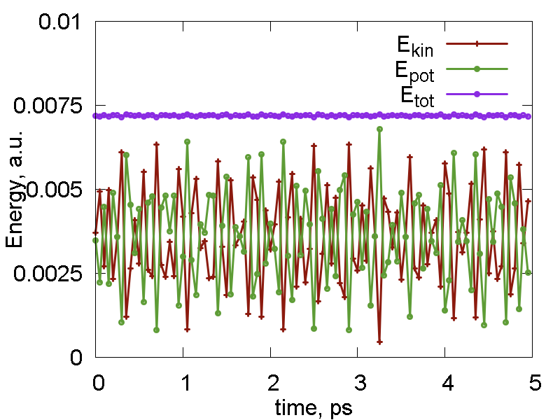
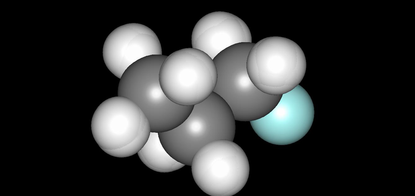
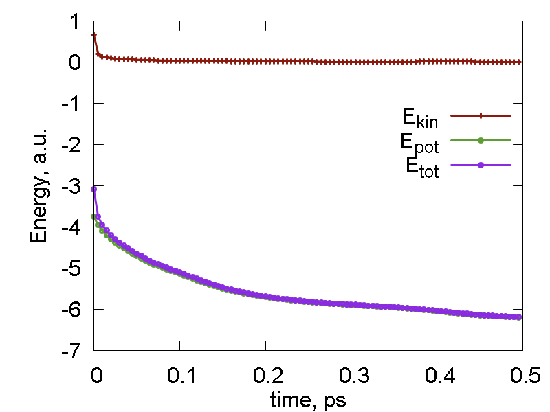
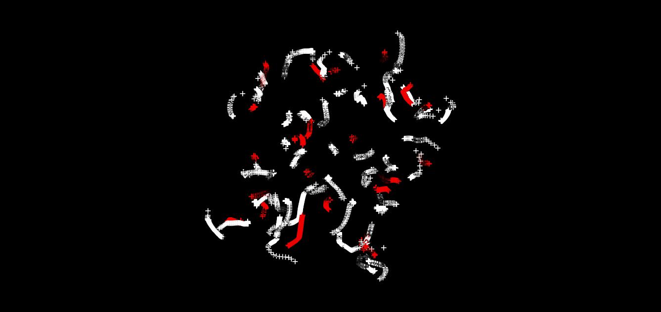
This tutorial script is merely the cleaned up (no excessive information print) version of the previous one. In addition, we have used nested loops to print out the coordinates every 100 steps (each step is about 0.5 fs). The energetic properties (potential, kinetic, total energies) are printed every step. The total number of steps is 100 x 100, which os 5 ps. The energies are plotted in Fig. 1a. Fig. 1b shows the overlay of the 100 configurations of the system over its evolution. One can see that there are certain fluctuations of the hydrogen atoms, whereas the carbon and fluorine nuclei remain almost fixed. This difference originates from the masses disparity.
a
b
test_mm6.py
Earliear, we have mentioned that the objects of "System" class (in our case it is the "syst" variable) serves mostly for representing chemical system, its properties and for manipulations on that system. However, the class contains all variables needed for describing the dynamics of the system. Here, we show how to use them as the dynamical variables. In addition, we will show one of the important methodological features available in the Libra code - the rigid body MD (RB-MD).
-
First, lets define our system. This time, we use the cluster of 23 water molecules. If we look into our file, we will find the definition of the fragments:
GROUP    1   2   3       FRAGNAME  WAT  O  H  H
GROUP    4   5   6       FRAGNAME  WAT  O  H  H
GROUP    7   8   9       FRAGNAME  WAT  O  H  H
GROUP   10  11  12       FRAGNAME  WAT  O  H  H
...
The format is pretty simple - the keyword "GROUP" followed by the list in integers (which are the ids of the atoms included in this group), followed by the "FRAGNAME" keyword, the name of the group and by 3 literals which have no special meaning so far. In the present example, the fragmentation scheme is pretty straightforward - each water molecule is treated as a separate rigid fragment. All internal bond stretching and angle bending modes are frozen. -
There are no bonded interactions among the atoms of different water molecules, it is crucial to include non-bonded interactions in our computational scheme. Earlier we have said about the limitations of the 2-body vdW and electrostatic terms. Here, we show how these types of interactions should actually be included. For this purpose, we add a many-body potential - see the last line:
uff = ForceField({"bond_functional":"Harmonic",
"angle_functional":"Fourier",
"dihedral_functional":"General0",
"oop_functional":"Fourier",
"mb_functional":"LJ_Coulomb","R_vdw_on":10.0,"R_vdw_off":15.0 })
One can also see how the cutoff parameters for vdW interactions are defined. The "LJ_Coulomb" interaction potential takes care of both vdW and electrostatic interactions in our system. Another new feature we find in this script is:
syst.init_fragments()
This function is essential when we work with fragments larger than 1-atomic. This is needed because the function computes basic properties of the fragments - their masses, inertia tensors, internal coordinates, centers of mass, total moments, etc.Before we can start actual propagation, we still need to initialize Hamiltonian-dependent rigid-body properties. These are total forces and fragment torques. The "init_fragments" function does take care of this, but if it is called before atomic forces are zero, the total fragment forces and torques are zero. Thus, we call this function one more time (actually, we could call it only here, but the point is to show the difference - for the purposes of this tutorial) after the function "init_md" is completed.
The "init_md" is an auxiliary function we define right in this Python script. What should be emphasized here, is the way new functions exported from the Libra package are called in there. We already know several, so we briefly discuss 3:
syst.Fragments[n].Group_RB.ekin_tr()
syst.Fragments[n].Group_RB.ekin_rot()
These are the two functions of the RigidBody (from the "libdyn") class. Apparently, they return translational and rotational contributions to kinetic energy of each fragment.syst.zero_forces_and_torques()
This instruction is very important, although it is very simple. It merely nullifies the forces and torques of all rigid fragments. Moreover, it also sets to atomic forces to zero for all atomis in the included fragments. The calculations in Hamiltonian_Atomistic are organized in the way that simply adds new forces to corresponding places. This is needed, so that initialization inside of one type of Hamiltonian (e.g. QM) would not discard forces computed in another part (e.g. MM). So, the forces are simply added to one place. Thus, it is important to clean that space before we start computing all contributions to forces.syst.update_fragment_forces_and_torques()
The forces computed by the "compute_forces(mol, el, ham, 1)" procedure are the atomic forces (converted from "mol" structure to the "syst" object via "syst.set_atomic_f(mol.f)" procedure). However, the total forces acting on the centers of mass of the fragments and the torques are not computed automatically. The above instruction does this for us.In the integration cycle, we do a little dance between different variables, including force initialization (to zero) and updates:
syst.zero_forces_and_torques()
syst.extract_atomic_q(mol.q)
epot = compute_potential_energy(mol, el, ham, 1)
compute_forces(mol, el, ham, 1)

syst.set_atomic_f(mol.f)
syst.update_fragment_forces_and_torques()
- Finally, in the integration, we use the Verlet-type scheme for translational DOF, using the corresponding functions and data members
of the "RigidBody" class:
syst.Fragments[n].Group_RB.apply_force(0.5*dt)
syst.Fragments[n].Group_RB.apply_torque(0.5*dt)
...
syst.Fragments[n].Group_RB.shift_position(dt * syst.Fragments[n].Group_RB.rb_p * syst.Fragments[n].Group_RB.rb_iM)
...
Integration of orientational DOF is done with one of the RB-MD integrators:# Propagate rotational DOFs if integrator=="Jacobi": syst.Fragments[n].Group_RB.propagate_exact_rb(dt) elif integrator=="DLML": ps = syst.Fragments[n].Group_RB.propagate_dlml(dt)In this example, only two methods are shown. For the complete list refer to RigidBody.h file. - Perhaps, the last note about this test script is the following. Once the have updated orientations of the rigid bodies and the positions of
their centers of mass, we need to translate these changes into the changes of Cartesian coordinates of all atoms included in updated fragments.
This is done with the following snippet:
for n in xrange(syst.Number_of_fragments):
    syst.update_atoms_for_fragment(n)
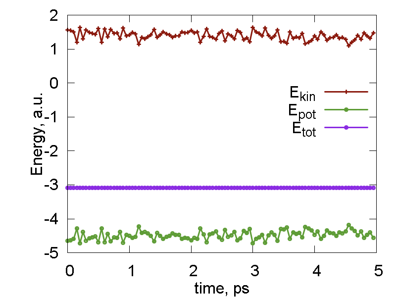
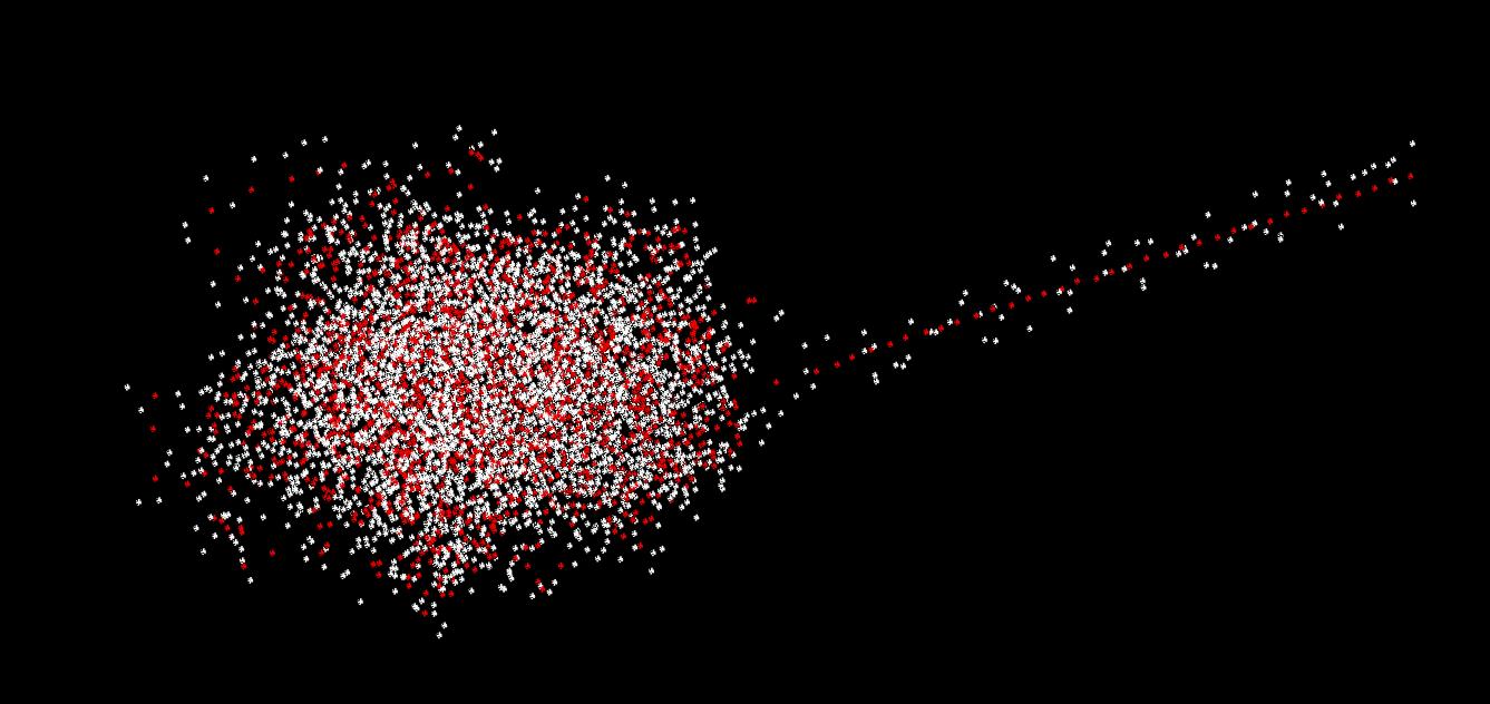
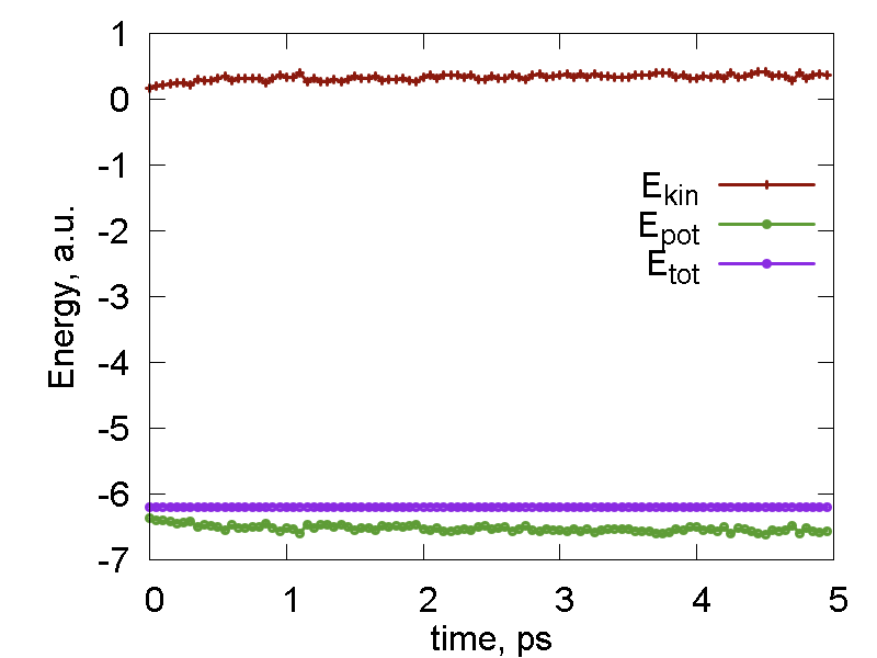
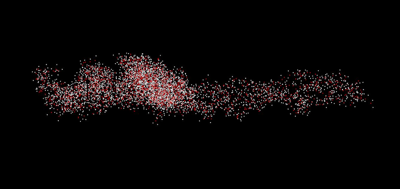
The results of our 5 ps simulations (100 rounds, each 100 steps of 0.5 fs long) of the 23 water molecules are shown in Figure 2. We can see that the cluster stays stable, even though the kinetic energies are very large. We can observe only one molecule moving away from the rest of the cluster (the dotted line (oxygen) with spirals (hydrogens)). Nonetheless, the total energy remains constant and does not show any notable drift.
a
b
test_mm6a.py
This tutorial is based on the previous one. It shows how we can organize our computations in a more modular and convenient way. Basically, we have taken the main portion of the integration procedures and formed an auxiliary Python function "md_step". Why? Well, the main rationale is that we can reuse it in different contexts, but we don't want to increase the size of our script.
As for the places where the new "md_step" function is used. As you can see, the propagation section now contains two logical partitions. In each partition we perform RB-MD simulations, but in the first one we also cool our system periodically. This is done via:
syst.cool()This function simply sets momenta of all atoms and the linear and angular momenta of all rigid bodies to zero. Obviously, this is the way to remove excess temperature from our system. When we alternate this with our normal RB-MD steps, we allow system to gradually find the potential energy minimum. In the MD steps, the potential energy can convert into the kinetic energy. When the latter is taken away in the cooling step, the total energy of the system decreases, and the phase space reagion which the system can explore decreases. Eventually, this procedure converged to a single point which has minimal potential energy. This approach is essentially that of the simulated annealing.
The cooling rate may be a critical factor. If the we take the excess of energy away sufficiently slowly, the system can explore bigger region of the phase space. Therefore, the chances to find the global minimum increas. If the cooling rate is too large, the system would technically be following the direction opposite of the gradient, so it would reduce to the steepest descent minimization. In this regime, it is more likely that the system would end up in one of the local minima.
As we can see, the combination of MD and cooling works essentially as an optimization algorithm. This is what the first logical section is. In our case, we perform 100 cycles of optimization. Each cycle consists of 10 MD steps followed by cooling. The energy evolution and the overlay of 100 nuclear configurations for this step are shown in Fig. 3 (panels a and b, repsectively). One can see that the total energy is almost always equal to the potential energy (except for the very beginning of the simulation), both decaying. This is exactly what we expect - the energy optimization in action. The kinetic energy is large initiall decays fast to zero. Because each round consists of only 10 steps and because we always freeze the nuclear motion, the overlay of the configurations in not that busy as in Fig. 2b, for instance. This overlay is essentially a rendering of the multidimensional representation of the converging trajectory.
The optimization is followed by the normal MD simulation with the same parameters as in the previous two RB-MD examples. The energies and trajectory are shown in Fig. 3c and 3d, respectively. Note that the kinetic energy of the system is now much lower that what we had in the previous (unoptimized) example. Also, no molecules fly away from the cluster. Instead, all molecules fluctuate much less than in the previous example. One can even recognize the maxima of probability density to find atoms of different types. This way, one can identify individual water molecules, in contrast to much more busy picture Fig. 2b.
a
b

c
d
test_mm6b.py
This is example is essentially RB-MD without optimization. The only point of this test is to show that the initial momenta/angular momenta can be initialized to have a certain values, that can be consistent (to certain extent) with the given temperature (total kinetic energy) and the directions of total angular and linear momenta of the entire system. This is done with the function
syst.init_fragment_velocities(300.0, VECTOR(1.0, 0.0, 0.0), VECTOR(0.0, 0.0, 1.0) )Here, the first vector defines the total linear momentum of the system, whereas the second one defined the total angular momentum of the system.

a
b
Figure 4 show the trajectories of 23 water molecules (5ps, 0.5 fs time step, 100 snapshots) computed with two initial conditions: Px=1, Lx=1 (Fig. 4a) and Px=1, Lz=1 (Fig. 4b). One can see qualitatively different trajectories. In the first case, the combination of the translation of some molecules along positive x direction (and some along negative) and rotation around this axis lead to formation of spiral many-particle trajectories (several molecules' motion creates such spirals). In the second case, one obtains more of a ball, although one can recognize several molecules movig around the z axis, of the ball - like the sattelites around a palnet.