Libra: An open-source "Methodology Discovery" Library

Libdyn Tutorials

The "libdyn" is a module that implements a number of classes to represent different dynamical degrees of freedom (DOF) and compute their evolution (propagate).The working files showing how to use different objects are located in the /tests/test_dyn directory of the Libra package. Most of the tutorials are almost completely self-explanatory. Here, we only focus on most interesting/less straightforward conventions and articulate some of our actions.

test_nuclear.py

Lets start with something relatively simple - classical integration of the 1-D models: a) Harmonic oscillator; b) Morse potential. For each problem, we define the ppropriate function - right in the Python script: pot and pot2. The functions take the coordinate of the particle as argument and return forces and energy as output.

For each problem we create an object, "mol" of the "Nuclear" class:

mol = Nuclear(1)
mol.mass[0] = 2000.0
mol.q[0] = 1.0
mol.p[0] = 0.0

The argument 1 supplied to the constructor implies that we have only 1 nuclear DOF (by the way, don't confuse it with the 3-D vector describing a single particle in 3D space. No - we only have 1 component, e.g. x). The object contains all the necessary dynamical information to describe nuclear DOF - mass, position, momentum, force. These properties are arranged in an array with the number of elements equal to the number of nuclear DOF. In our case, there is only 1 DOF, so we access only the 0-th element: mol.mass[0], mol.q[0], mol.p[0], mol.f[0], respectively.

Nuclear dynamics is then propagated using Verlet scheme, which is implemented via the following sequence of operations:

mol.propagate_p(0.5*dt)
    mol.propagate_q(dt)
    mol.f[0], epot = pot(mol.q[0])
    mol.propagate_p(0.5*dt)

The "propagate_*" functions are very simple - they simply shift the variables by the amount proportional to the argument and also other internal variables. The argument is the integration time step, dt. But because Verlet scheme is symmetric, one of the variables (usually momentum) is propagated twice for the magnitude proportional to half of the integration time step. The force and potential energy depend on coordinate, so they are updated after each update of the coordinate. Eventually, the overall integration step is finished with the computation of the kinetic energy of the system by calling:

ekin = compute_kinetic_energy(mol)

As you can see, each sequence of steps is repeated for 500 times. This means we perform 500 integration time steps of size dt = 1.0 As other purely Pythonic instructions suggest, we print the dynamical variables and other properties (energies) for each time moment. The data can then be plotted (in my case, i use gnuplot), to visualize some dynamical characteristics. In particular, below we show the evolution of kinetic, potential, and total energies for harmonic oscillator (Fig. 1a) and Morse potential (Fig. 1b). Note that the total energy is conserved very well in all cases, implying the integration scheme and the choice of integration parameters (dt = 1) are both good. We also show the evolution of the system in the phase space spanned by the coordinate q and momentum p - for harmonic oscillator (Fig. 1c) and Morse potential (Fig. 1d).

test_nuclear2.py

In addition to manually-defined Python codes for computing energy and potentials, it is possible to use the pre-defined potentials. Here, we will consider such potentials - model Hamiltonians. Model Hamiltonians are represented by the class "Hamiltonian_Model". So to construct an object of this type for further use, we do:

ham = Hamiltonian_Model(1)  # DAC
ham.set_rep(1)  # adiabatic

The constructor Hamiltonian_Model takes a single integer as an argument. The argument selects one of the predefined models and sets up some deafult parameters and appropriate dimensionalities. In our case, the numebr 1 selects the double avoided crossing (DAC) problem of Tully. The model implies one nuclear DOF and 2 electronic. Once the Hamiltonian object is created, it is important to setup the representation. This is done in the second line of the code. The number 0 selcts the diabatic representation, 1 - adiabatic representation, so in our case we select the adiabatic representation. This setting will be used later - when actual calculations will be performed.

The calculations involving model Hamiltonians require electronic DOF be defined, even if a simple ground state (adiabatic) nuclear dynamics is performed. To define electronic DOF, we use the constructor of "Electronic" class:

el = Electronic(2,0)

This instruction creates and object "el" that represents electronic DOF. The first argument "2" of the constructor defines the number of electronic DOF. The second argument defines how to initialize the electronic DOF. In our case, "0" makes the first electronic state (ground state) populated. This means that the member data ".istate" that contains the discrete index of the state (e.g. for surface hopping) will be set to 0 and the amplitudes of the 0-th electronic DOF will be set to have magnitude of 1 and random phase. All other amplitudes will be set to zero.

Nuclear DOF are initialized similar to how we did it in the previous example. The integration scheme is also exactly the same as in the previous example. The only difference with the former case is in the way we compute energies and forces. Instead of Python-defined function (which, by the way, may often be easier to modify), we call the functions "compute_potential_energy" and "compute_forces":

epot = compute_potential_energy(mol, el, ham, 1)  # 1 - FSSH forces
compute_forces(mol, el, ham, 1)

As you can see, both functions take the same 4 arguments: mol - the object that contains the nuclear DOF, el - the object that contains electronic DOF, and ham - the Hamiltonian object (the functor) which handles all calculations for all electronic states - it computes vibronic Hamiltonian. The final argument is an integer that defines the way energy and forces are computed - it controlls the effective Hamiltonian. In our case, the integer is set to "1", which corresponds to state-specific energies and forces. In the nonadiabatic MD simulations this would correspond to FSSH-type treatment of energies and forces. The alternative option is "0", in which case the mean-field (Ehrenfest) type of treatment will be performed.

Note that all objects are passed by reference, which is very convenient - the function "compute_forces" modifies the corresponding data members of the "mol" object. Thus, we utilize a procedural/functional approach, when a function works as a sort of "factory" - it takes some object, uses its data, but also modifies the object itself. As another note, one in principle could use only one of these functions - "compute_forces", becuase it returns the required potential energy:

epot = compute_forces(mol, el, ham, 1)

Here, we only demonstrated that it is possible to compute only energy without doing additional costly computations of gradients - one can use the "compute_potential_energy" function.

Finally, the in Fig. 2 we show the evolution of kinetic, potential, and total energies (Fig. 2a) and the phase space trajectory (Fig. 2b) of this system.

test_electronic.py

Above we have used the objects of class "Electronic". The present script demonstrates several ways to initialize the object of such type (different constructors) and also demonstrates different member data. Specifically:

• Electronic() - (default constructor) one electronic DOF is reserved - good for any ground-state calculations
• Electronic(n) - (constructor) reserves n electronic DOF, system is in the lowest state (index 0)
• Electronic(n,i) - (constructor) reserves n electronic DOF, but sets the system to be in i-th state
• el.istate - (member) the indeger index labeling current state in which the system exists right now
• el.nstates - (member) the number of electronic DOF (the number of electronic states)
• el.q[n], el.p[n] - (members) the MMTS mapped variables that describe dynamics of electronic DOF n. Related to complex amplitudes of all states as: c = q + i*p, where i - is the complex unity
• el.c(n) - (member-function) - returns the complex amplitude of the quantum state n
• el.rho(i,j) - (member-function) - return the complex (in general) elements of density matrix, i - row, j - column: rho(i,j) = c^*_i * c_j Only the diagonal elements (populations) are real.

test_el_dyn.py

Now, when we have familiarized ourselves with the structure of the electronic variables (objects of type "Electronic"), we can learn how it can be used in propagation schemes. The propagation of electronic DOF is based on solving semiclassical TD-SE, i*hbar*dc/dt = H*S*c. In our implementation we use the mapped variables q and p, so the TD-SE reduces to the pair of Hamiltonian equations of motion. So we apply a symplectic scheme based on symmetric Trotter factorization of the evolution operator. This scheme is implemented in the "propagate_electronic" function with the latter called as:

el.propagate_electronic(dt, ham)

The function is the member-function of the Electronic class. It takes two arguments as inputs: dt - the integration time step, and ham - the Hamiltonian object which handles computations of energies and couplings.

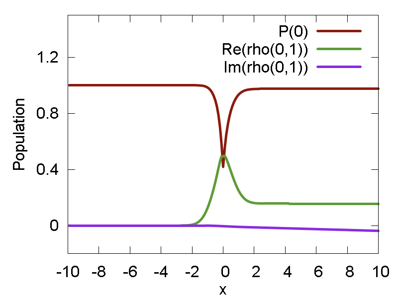
Unlike the previous example, where the all computations with ham object were hidden in the "compute_forces" or "compute_potential_energy" functions, here we explicilty call those calculations. In the first example of this script we use the single avoided crossing model Hamiltonian of Tully (this is selected by choosing "0" in the constructor). For this problem we choose adiabatic representation:

ham.set_rep(1)

Moreover, we since the purpose of this test is to show the integration of electronic DOF, we don't care much about the nuclear dynamics and choose the simplest (although not very physical) approach - to assume that the momentum of the particle is fixed, so the particle is moving along x direction uniformly (despite that the potential energy is not flat). Thus, instead of Verlet-type integration, we get the motion law x(t) = x(0) + v*t. Because we assume the velocity is constant, we let the Hamiltonian know this only once - before the loop over time, via:

ham.set_v([v])

Although the electonic Hamiltonian does not depend on velocities, the vibronic Hamiltonian in adiabatic representation does contain the dependence on velocity - via the nonadiabatic coupling terms. Thus, it is important to take reset velocities every time they change, if the adiabatic representation is used. But, again, in our simple example we assume the velocity is constant, so we set it only once.

The potential energy and couplings do depend on the coordinate. The coordinate changes linearly with time, so we need to tell Hamiltonian that the coordinate changes every iteration. This is done via:

ham.set_q([x])

Finally, once the velocity (for adiabatic case) and coordinate (both for adiabatic and diabatic cases) are set, one can invoke computation of the corresponding vibronic Hamiltonian (selected by the ser_rep() function) via:

ham.compute()

For the model calculations, the updated vibronic Hamiltonian is stored internally, and then its elements are acessed to integrate evolution of electronic DOF in the "propagate_electronic" function.

The evolutions of SE populations and coherences along the predefined path is shown in Fig. 3a. One can see that the SE population changes drastically as the particle passes x = 0 region. That is expected, since this is where the nonadiabatic coupling is large, causing large population transfer. In addition, the coherence changes at this point - especially its real component. The coherence, once developed, does not decay in this method. Thus, the SE describes system at t = +inf as a coherent superposition of the two states.

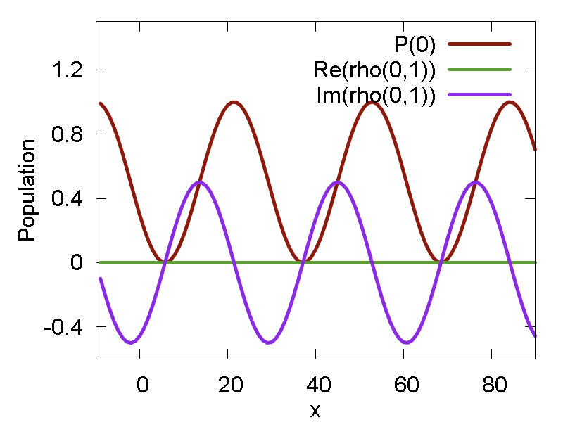
The second example in this script shows 2 things: a) that the computations can also be performed in the diabatic representation; b) how the parameters of the model Hamiltonian can be manually set with

ham.set_params([0.1, 0.1, 1.0])

Note that the model is also different - now it is a simple 2-state Rabi model. When transforming into adiabatic representation, the model would yields zero nonadiabatic coupling and show no population transfer between adiabatic states. In the diabatic representation, however, the population of the two diabats would oscillate. The same happens with the coherences, except that the real component of coherence is zero at all times. The plots of population of the lowest state and the components of the coherence are shown in Fig. 3b.

test_ehrenfest.py

Now, we are in position to make the previous electronic dynamics calculations to be more physically sound. Namely, we want to propagate the nuclei on the actual potential energy surface, and not to assume that the velocity is constant and motion is uniform, as in the previous example. Thus, we add the Verlet integration scheme to describe the dynamics of nuclei - as we did in one of the earlier examples.

The difference in our new Verlet integration scheme from the one we used before, comes in the choice of the option to comput effective Hamiltonian. In "compute_potential_energy" and "compute_forces" we pass the parameter "0", not "1" as before. Our present choice selects the Ehrenfest-type treatment of nuclear dynamics. In Ehrenfest (also known as mean-field, MF) approach, the nuclei muve in the average potential - the one which accounts for ground and all excited state surface, all taken with the corresponding SE weights.

Since the MF potential depends also on electronic veriables that are also propagated according to TD-SE (see previous example), and because the TD-SE solution depends on nuclear dynamics, the dynamics of electonic and nuclear DOF are coupled self-consistently. All the components of the integration scheme have been discussed in the previous sections.

Perhaps, it is important to remind again that since in this example we use adiabatic representation, it is important to tell the Hamiltonian to take the updates of velocities into account - before effective Hamiltonian and forces are computed. This is done via "set_v()" function.

The results of Ehrenfest dynamics are presented in Fig. 4

One can observe that total energy of the system conserves pretty well, even though the potential and kinetic energies change significantly. The only potentially problematic place, where integration must be carried out carefully is close to the conical intersection regions, where the nonadiabatic coupling becomes very large. In the DAC, there are two such points. When particle passes them, we can observe some fluctuations of the total energy. Yet, no overall trends or deviations of the total energy is observed on the whole scale of simulation, indicating the stability of gives simulation.

Fig. 4b shows how the populations and coherence (square of its magnitude) change along the trajectory. One can clearly see two almost step-wise changes of the populations: These changes occur at the points of strong nonadiabatic coupling (each of the avoided crossings). At the same points the coherence develops. The coherence evolves periodically and doesn't decay.

test_tsh.py

We move further to trajectory surface hopping (TSH) calculations - an alternative to Ehrenfest approach. The first example will show the evolution of different properties along a single random trajectory. We will showcase some other functions available in "libdyn" module.

In general, the most part of the script follows that in the "test_ehrenfest.py" - we again perform simulataneous integration of TD-SE and evolution of nuclei. The first difference comes in the option for "compute_forces" and "compute_potential_energy" functions. We choose "1" to use state specific forces. However, unlike the ground state (classical MD) examples discussed in the beginning of this tutorial, we will be able to actually switch between the states. Remember, last time we stayed on the ground state no matter what. The switching of the states in the present algorithms is what gives the name to the "TSH" group of methods - our trajectory will be able to hop between states. Once it has hopped to a given state, the nuclear dynamics will be governed by the forces (and energies) specific to that particular state.

The second difference comes in the section that computes surface hopping probabilities:

g = MATRIX(2,2)
# Just choose the TSH scheme below
#compute_hopping_probabilities_mssh(mol, el, ham, g, dt, use_boltz_factor, T)
compute_hopping_probabilities_fssh(mol, el, ham, g, dt, use_boltz_factor, T)
#compute_hopping_probabilities_gfsh(mol, el, ham, g, dt, use_boltz_factor, T)
		

Here we first create a 2 x 2 matrix "g". Then we call one of the 3 functions - each computes surface hopping probabilities according to specific algorithm: FSSH (fewest switches surfac hopping - this is the original Tully's surface hopping algorithms), GFSH (global flux surface hopping), or MSSH (Markov-state surface hopping). All functions take similar arguments: "mol" - the variable containing the state of nuclear coordinates, "el" - analogous variable containing state of electronic DOF, "ham" - the Hamiltonian functor, "g" - the matrix which will be populated with the surface hopping probabilities to go from one state to another, "dt" - the nuclear integration time step, "use_boltz_factor" - the flag choosing how to treat frustrated hops (or rather how to implement them), to provide a means to describe proper distribution of populations at thermal equilibrium, "T" - the effective nuclear temperature. First, lets talk about "g". Remember, objects are passed in Python by references. And that is what we use here. We pass the object "g" to function "compute_hopping_probabilities_*" and collect appropriate values in it. The matrix element g.get(i,j) gives the probability to hop from state "i" to state "j". The diagonal elements, g.get(i,i), are of course the probabilities to stay on the state i (not to hop anywhere). The next new parameter is "use_boltz_factor". In our present example it is set to 0, to indicate that the standard hop rejecttion criterion based on the total energy conservation is used. In some atomistic calculations withing the classical path approximation, the nuclear trajectory is predefined. This means that one can't apply the energy-conservation hop rejection criterion and can't rescale velocities afterward the successfull hop. Instead, the probabilities to hop to a higher energy level E_j from a low-energy level E_i are rescaled by the Boltzmann factor exp(-(E_j - E_i)/kT). The effective temperature, T, is given by the last parameter passed to the above functions.

The third and the last major change in this script with respect to the one describing Ehrenfest dynamics is the following block:

do_rescaling = 1 
do_reverse = 1
rep = 1 # adiabatic
ksi = rnd.uniform(0.0, 1.0)
el.istate = hop(el.istate, mol, ham, ksi, g, do_rescaling, rep, do_reverse) 

These are the instructions that actually use the just computed hopping probability matrix "g" to decide wheter or not to change the integer state of the electronic DOF (the memember "istate"). This is done withing the function "hop()". The function returns the integer index of the electronic state - whether new (hop has happened) or old (no hop, or hop was not accepted).

The hop is a stochastic process. It is made using random number generators. Libra implemnts a number of random number generators, which can be used after creating an object of class "Random". This is actually done in the beginning of the script in the line:

rnd = Random()

Once the random number generator is created, we can call it to produce a random number taken from needed distribution. In our eaxample we draw the number uniformly distributed on [0,1]. This random number is then used in the "hop()" function as a stochastic input. Because of the stochasticity, one typically needs to run large number of trajectories to get statistically-meaningful results. This tutorial runs only a single trajectory, thus the sucess of the hop may strongly depend on your luck at the moment. If you don't see transition, just run the calculation again.

Important note about random numbers generator: Note that in our simulation (withing all loops) we only call rnd.uniform(0.0, 1.0), but do not construct new ojects of "Random" class. This is very important for getting proper results, because the creation of new "Random" object means that the intrinsic random number generator will be reseeded every time the "rnd" object is created. The seeding is usually attached to time. Since the computations are very fast, the two consequtively seeded random number generators will generate practically same sequence of numbers. This effectively would translate into the only "random" number being thrown all the time. This can significantly deteriorate the statistical properties of the calculations performed. Thus, it is important to create the "rnd" object only once!

In the passing, let us comment of the 3 other parameters. First, "do_rescaling" - this is the flag that chooses whether to rescale the velocities after successfull hops, to conseve total energy (=1) or not (=0). The latter choice would be consistent with the "use_boltz_factor = 1" withing the CPA tratment. Second, "do_reverse". This option controls what to do with nuclear momenta when frostrated hops occur. If the choice is 1, the momenta will be reversed; if the choice is 0, the momenta will be left unchanged. Third, "rep" - this is the representation in which we work (0 - diabatic, 1 - adiabatic). In this context, the representation is needed to choose proper algorithm for velocity adjustment. In the adiabatic representation, the momenta will be rescaled in the direction of corresponding derivative coupling vectors, according to the original prescription of Tully. In the diabatic representation, the direction of the momenta will not be changed, only their magnitude will be adjusted to conserve the total energy.

The results computed for 1 FSSH trajectory are shown in Fig. 5. The energy is well conserved, even when the hop occurs (Fig. 5a). The populations and coherences (Fig. 5b) evolve similar to those shown in the previous example (Ehrenfest) - this is the consequence of sufficiently large initial momentum. It is likely that more notable differences will be observed in the low-momentum cases, when quantum effect will be stronger. One can also observe that the variable describing the integer state "istate" changes abruptly (hop) from 0 (lower state) to 1 (upper state) - Fig. 5c. In addition, we also show the phase space trajectory (a similar one is obtained in the Ehrenfest dynamics) - Fig. 5d.

test_tsh2.py

So far, the TSH calculations have been performed for a single trajectory. Although we have seen the change of the discrete state, the statistics was far from enough. This means, only sufficiently large number of independent trajectories make sense, not a single one - one has to have sufficient statistics of surface hops. Thus, we need to run a series of the calculations to get such statistics. Although it is possible to use the tools and classes we have already introduced (and that will be shown in later examples, when i get to that point), here we want to demonstrate yet another class designed for performing such statistical calculations. The class is called "Ensemble", and as the name suggests, it represents an ensemble of trajectories - that is a collection of electronic and nuclear DOF and corresponding Hamiltonians for each copy/replica of the system.

The ensemble of ntraj=50 trajectories, each of which involves 2 electronic states and 1 nuclear DOF can be created using the constructor:

ens = Ensemble(ntraj, 2, 1)

The electronic and nuclear DOF are stored in the member-data array: "el" and "mol", respectively. These elements (and hence some of their internals) can be accessed directly, as for instance in the following instructions:

for i in xrange(ntraj):
    # Nuclear DOFs
    ens.mol[i].mass[0] = 2000.0
    ens.mol[i].q[0] = -10.0
    ens.mol[i].p[0] = 20.0
		

or

ens.el[i].istate = hop(ens.el[i].istate, ens, i , ksi, g, do_rescaling, rep, do_reverse)  

However, the Hamiltonians are not stored as objects. Instead, the "Ensemble" class stores the array of pointers to the objects of class "Hamiltonian". Note, that this is the base class of the derived "Hamiltonian_Model" and "Hamiltonian_Atomistic". This allows one to assign those pointers to model or atomistic Hamiltonians, respectively. Therefore, the dynamical procedures can be used in the exactly same manner for both types of calculations. Since we store the pointers, it is very problematic to access pointers from the Python environment. Thus, the modifications of the Hamiltonian properties are done via the mathods. These methods, defined in the "Ensemble" class also take the index of the element of the array we want to access - again, this is because we deal with pointers rather than with instances (object), so the indexing and element access get a bit more complicated here.

The methods we have seen in the previous script to affect the Hamiltonians are exported in the interface of the "Ensemble" class, so we can do:

ens.ham_set_v(i, [ens.mol[i].p[0]/ens.mol[i].mass[0]] )

This example shows that we can access the properties of specific Hamiltonians

The methods for propagation of electronic and nuclear DOF are now applied to all trajectories of the ensemble, which simplifies the scripting (so we don't need to write additional loop over all trajectories in the ensemble), like here:

ens.el_propagate_electronic(0.5*dt)
ens.mol_propagate_p(0.5*dt)
ens.mol_propagate_q(dt)
ens.ham_set_v()
		

The functions for computing the energies and derivatives are overloaded to take the object of the "Ensemble" class as an argument (by reference!):

epot = compute_potential_energy(ens, 1)  # 0 - MF forces, 1 - FSSH
compute_forces(ens, 1)
ekin = compute_kinetic_energy(ens)

A thought of the future design. In fact, we should be able to simply set the correspondence between internal pointers (stored inside the "Ensemble" class) and the objects created in the Python script. Then, we should be able to simply modify the objects with the normal methods of the "Hamiltonian" class. Since the pointers of the "Ensemble" class point to these objects, the changes of the seemingly detached objects would be included in the calculations done inside the methods of the "Ensemble" class. This would save us the hassle of exporting almost all methods of the "Hamiltonian" class also in the "Ensemble" class. But that is for future.

Since each trajectory realizes an independent stochastic hopping process, we individualize the dynamics at the point of hopping, so that the randomness is different for each trajectory. This is realized via using the overloaded version of the "hop" function - the one that takes the argument of "Ensemble" type and the index of the trajectory to work on. This is shown in the following snippet:

for i in xrange(ntraj):
    # Just choose the TSH scheme below
    compute_hopping_probabilities_mssh(ens, i, g, dt, use_boltz_factor, T)
    #compute_hopping_probabilities_fssh(ens, i, g, dt, use_boltz_factor, T)
    #compute_hopping_probabilities_gfsh(ens, i, g, dt, use_boltz_factor, T) 

    ksi = rnd.uniform(0.0, 1.0)
    ens.el[i].istate = hop(ens.el[i].istate, ens, i , ksi, g, do_rescaling, rep, do_reverse) 
		

This script also demonstrates two member-function of the "Ensemble" class - the functions for computing the statistics of the ensemble - both in terms of average TD-SE populations of different states, as well as the average TSH populations.

se_pops = ens.se_pop()
sh_pops = ens.sh_pop()

The functions return the lists with the populations of all electronic states for given state of the ensemble.

The evolution of SE and SH populations for the DAC model and given value of initial nuclear momentum is presented in Fig. 6

test_tsh3.py

In this example, we simply repead what our previous script does - but just for different initial conditions (initial momenta). This done by repeating the code from the previous example, inside of the loop that changes initial value of the nuclear momentum. We also take care of proper re-initialization of the ensemble object - for each new initial momentum. We focus only on the total populations of electronic states, do not resolve them spatially. The computed probabilities are shown in Fig. 7.

test_tsh4.py

In this example, we go even further. This script is the improvement of the previous one along the 3 following lines:

• Main change for this example: we resolve probabilities depending on spatial location of the trajectories, so we can judge on the reflection/transmission probabilities on different states. This is done with one of the overloaded versions of the "se_pop", and "sh_pop" functions. This is demonstrated in:

  se_pops_tr = ens.se_pop(0.0, 100000.0)
  sh_pops_tr = ens.sh_pop(0.0, 100000.0)
  se_pops_re = ens.se_pop(-100000.0, -0.0)
  sh_pops_re = ens.sh_pop(-100000.0, -0.0)
  

  Here, the arguments define the boundaries of the box in which the trajectory (each coordinate) should be confined. In our case, everything below 0.0 corresponds to reflection, above 0.0 - to transmission.
• The second improvement (minor): is the addition of the option to perform selected type of surface hopping. This is instead of manual commenting/uncommenting of the appropriate methods, as we did before.
• Finally, the thrid improvement (but this is mostly the development feature) corresponds to adding of the entangled surface hopping scheme (ESH) Methodologically, it is still under the development. What is important is that now the function takes the entire ensemble of the trajectories to compute hopping probabilities, decide on whether do hops or not, to actually perform the successfull hops, and to perform post-hop adjustments. Therefore, there is no additional loop over the different trajectories:

  compute_hopping_probabilities_esh(ens, g, dt, use_boltz_factor, T)

  Here, the variable "g" is not actually used - it is only here to preserve the signature of the function, to look similar to other surface hopping schemes. Like I said, the method implements some ESH scheme (under the development), so don't rely on it too much. Instead use it as a placeholder to implement new techniques. In the ESH methods, what is important is that the faith of all trajectories on the next time point depends on the state of all trajectories at the present time point. Therefore, we propagate (including surface hops) the whole ensemble as a single object. The disentangled schemes like FSSH and so on are just special cases of the "Ensemble" when entanglement is turned off. Yet, the scheme remains the same.

Here, we show the spatially-resolved scttering probabilities computed for the extended coupling with reflection (ECWR) model of Tully:

test_ehrenfest_extern.py

In this tutorial we will demonstrate a new feature of the Libra (first introduced on 12/27/2015) - the use of a new Hamiltonian type - the "Hamiltonian_Extern" class. The main purpose of this class is to enable calculations of the Hamiltonian and its derivatives right in the Python script, as opposed to hard-coded computations inside the Libra package.

This new capability may have many new uses. One that is most straightforward is the input of the Hamiltonians (energies and couplings) computed via the third-party codes. For instance, in our other package - PYXAID - we utilize a 3-step procedure for NA-MD. In the step 2, energeis and nonadiabatic couplings are computed for a given system. These quantities are printed in the files - two files per MD time step. In the step 3, one reads these files in and uses them to compute electronic dynamics (via TD-SE and surface hopping schemes). Now, the Hamiltonian_Extern class enbles creating of the Hamiltonians from the files generated in step 2 and performing NA-MD - right with the Libra components.

Another expected useage of the Hamiltonian_Extern class is in the methodology development. Namely, one can conveniently specify the Hamiltonians (or some effective ones) right inside the Python scripts. This may come along with the utilization of "normal" model or atomistic Hamiltonians. It is much easier to modify and tune the definition of matrix elements of the Hamiltonians in Python environment than to do this at the C++ level.

Now, let us show how this works.

First, we define (create) an external Hamiltonian and set up some important parameters:

ham_ex = Hamiltonian_Extern(2,1)  # 2 - # of electronic DOF, 1 - # of nuclear DOF
ham_ex.set_rep(1)  # adiabatic
ham_ex.set_adiabatic_opt(0)  # use the externally-computed adiabatic Hamiltonian and derivatives
		

The constructor takes two integers: first - the number of electronic DOF, second - the number of nuclear DOF. The constructor does not allocate any memory (well, almost no). The arguments are needed for further verification of the matrix bindings (see further). Basically, these arguments tell you what kind of input matrices to expect.

We are already familiar with the "set_rep" function. It choses the representation we are going to use in our calculations.

The next function - "set_adiabatic_opt" - is more interesting. Let us explain. This function sets up the internal variable (private) "adiabatic_opt". It controls the way the adiabatic Hamiltonian and its derivatives are "computed" in the Hamiltonian_Extern object. There are two ways. One option (when adiabatic_opt == 0, default) is to use the "read" adiabatic Hamiltonian as is, directly. The second option (adiabatic_opt==1), is to compute the adiabatic Hamiltonian from the "read" diabatic one. In the latter case, the adiabatic Hamiltonian associated with the Hamiltonian_Extern object may initially contain anything (e.g. all zeroes). Important: the adiabatic Hamiltonian still must be bound (associated). We will clarify the meaning of these "bound/associated" in the further discussion.

In the next lines:

# Actual matrices
ham_adi = MATRIX(2,2);  ham_ex.bind_ham_adi(ham_adi);
d1ham_adi = MATRIXList()

tmp = MATRIX(2,2)
d1ham_adi.append(tmp);  ham_ex.bind_d1ham_adi(d1ham_adi);
		

we actually allocate memory for the Hamiltonian (depending on situation, either diabatic or adiabatic or both) and its derivatives (respectively to the chosen representation). In fact, we never allocate memory for these quantities inside the Hamiltonian_Extern object. The whole point of this data type is that all memory is allocated externally. The modification of the allocated matrices is also performed externally. Now, if the objects are created externally, how does the Hamiltonian object knows about them and accounts for their changes (e.g. when calling H(i,j) or Hvib(i,j) functions)? Any guesses?..

Exactly, by reference! The base "Hamiltonian" class contains a number of pointers to the matrices (for Hamiltonians) and arrays of pointers to matrices (for derivatives). The only thing we need to do is to connect (bind) these pointers with the actual objects (external matrices). This is done with the range of "bind_*" functions, as in the above snippet. This way we don't need to manage memory inside of the "Hamiltonian_Extern" objects, and also account for any changes made to these matrices in the Python script.

In the above example, we use the adiabatic representation together with the adiabatic_opt = 1, which means we do not need diabatic Hamiltonians at all. Therefore, we only create the matrix to store adiabatic Hamiltonian - "ham_adi" and the list of matrices - "d1ham_adi" containing the derivatives of the adiabatic Hamiltonian w.r.t. all (1 in this case) nuclear degrees of freedom. We bind the two objects (of types MATRIX and MATRIXList) to the internal pointers using the "bind_ham_adi" and "bind_d1ham_adi" functions, respectively.

Now, as we solve the equations of motion, we need to update the matrices "ham_adi" and "d1ham_adi". In the present example, we actually use a "normal" model Hamiltonian object to recompute adiabatic Hamiltonian and its derivatives as the functions of nuclear coordinate.

# Update matrices
ham.set_v([ mol.p[0]/mol.mass[0] ])
ham.set_q([ mol.q[0] ])
ham.compute()
		

We next use the updated model Hamiltonian to change the "ham_adi" and "d1ham_adi" matrices:

for i in [0,1]:
    for j in [0,1]:
        ham_adi.set(i,j, ham.H(i,j).real)
        d1ham_adi[0].set(i,j, ham.dHdq(i,j,0).real)
		

Note, we don't do any manipulations with the "ham_ext" object. Yet, we use this object is all integration and computational procedures:

el.propagate_electronic(0.5*dt, ham_ex)
...
epot = compute_potential_energy(mol, el, ham_ex, 0)  # 0 - MF forces
compute_forces(mol, el, ham_ex, 0)
		

Eventually, you can see that the results obtained with this script coinside with the results obtained in the "normal" Ehrenfest example.