Libra: An open-source "Methodology Discovery" Library

Lattice Monte Carlo Tutorial

This tutorial shows how to utilize the Metropolis algorithm for Monte Carlo (MC) search of a minimal energy structure. In particutlar, we will consider 1D, 2D, and 3D cubic lattices composed of species of a given type. We then consider a certain percentage of doping of the lattice with species of another type. We then define the effective interaction Hamiltonian (lattice Hamiltonian) that relies on local coordination of each atom (site) of the lattice.

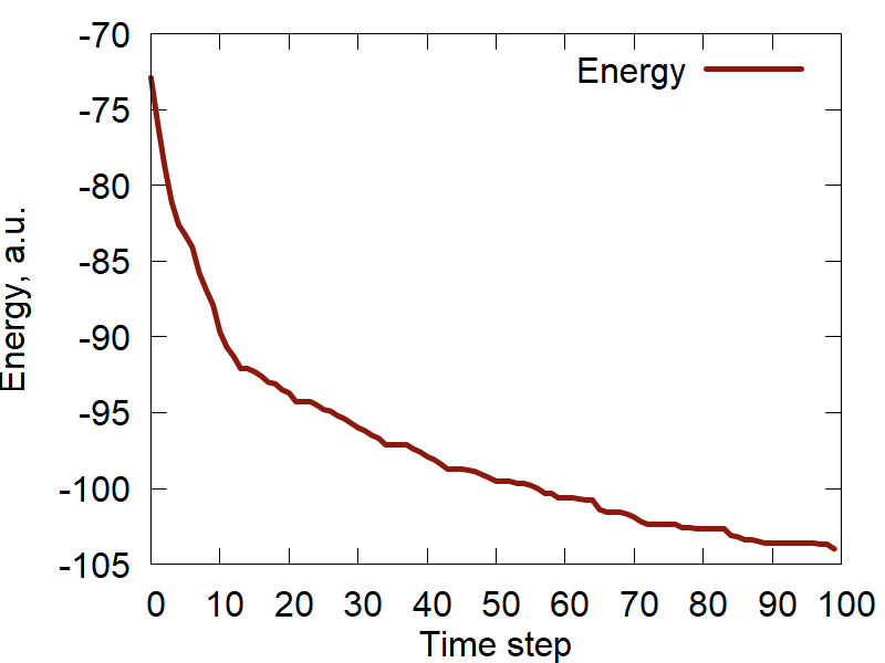
It is easy to realize that there are combinatorially-many configurations one could have. Thus, there is a multitude of configurations with local minium of energy, separated by high potential energy barrier. Direct optimization or even the MD-based sampling for minimal energy configurations (e.g. via annealing) would be computationally expensive and is not guaranteed to convergence to a minimal energy structure. Thus, the MC-based search for the minimal energy structure is the most optimal strategy, since it both has a potential of converging to the "global" minimum and may be made computationally inexpensive.

1. Create the folder where the snapshots of the configurations will be saved. E.g. mkdir 1D
2. Edit the input file with the unit cell composing the lattice, presently "ar.xyz"
3. Edit the file "model.py" according to the problem you solve
4. Execute the python script: python model.py
5. Edit the "make_pics.tcl" script, if necessary. E.g. to change the number of pictures to create
6. Switch to the created "1D" directory. cd 1D
7. In the VMD Tcl command line switch to the "1D" directory, e.g. cd "path-to-your-1D-directory/1D"
8. In the VMD Tcl terminal run the "make_pics.tcl" script by source ../make_pics.tcl

Script workflow overview

Lets look at the "model.py" script and explain the steps it is doing

First, we read a file containing the unit cell composition. The file is in the .xyz format. The assumption is the the coordinates are in Angstrom, but when we read it, they are converted to atomic units (Bohr) by the script. Notice that we use the "build" module of the "libra_py" module.

L0, R0 = build.read_xyz(prefix+".xyz")

Next, we define the lattice translation vectors and the number of translations in each direction and then create a supercell of a desired size. Vary the combination of Nx, Ny, and Nz to construct 1D, 2D, or 3D lattice. The example below shows how to construct a 2D lattice.

Nx, Ny, Nz = 30, 30, 1
a = VECTOR(1.0,   0.0,   0.0) * Angst # convert to a.u.
b = VECTOR(0.0,   1.0,   0.0) * Angst # convert to a.u.
c = VECTOR(0.0,   0.0,   1.0) * Angst # convert to a.u.
L1, R1 = build.generate_replicas_xyz2(L0, R0, a, b, c, Nx, Ny, Nz)

We define auxiliary variables - e.g. the masses and the maximal coordination number for all atoms. The masses are irrelevant for these calculations, so we set them just to 1.0. The MaxCoord variable is more important, because it will determine to how many nearby atoms (withing a specified radius) each atom of the lattice can be connected. The determined connectivities will later affect the calculations of the lattice energy. Note that the atoms (or rather the lattice sites) can be connected to fewer other sites, if there are not enough of them withing the bonding distance.

masses = []
MaxCoord = []
for i in xrange(len(L1)):
    masses.append(1.0)
    MaxCoord.append(6)

We are now ready to define the connectivities among the lattice sites. This is done with the help of the "autoconnect_pbc" function of the "autoconnect" module of the "libra_py" module. The autoconnect_pbc function takes as the arguments: 1) the positions of all sites (R1); 2) the maximal coordination number of each site (MaxCoord); 3) the bonding dinstance (Rcut) - if two lattice sites are separated less than this distance, they will be declared connected unless the maximal coordination number of any of the two sites is reached. In the latter situation, only the closest sites within the Rcut radius will be connected; 4) the translation vectors of the supercell (tv1, tv2, tv3) and the option for handling periodic connectivities (pbc_opt). These parameters are needed if we want to treat the lattice as periodic in any of the direction or in any combination of the periodic directions. In paricular, if one sets pbc_opt to "a", then the lattice will be treated as periodic in 1 dimension (a direction defined by the vector tv1). In that case, two lattice sites may be separated by more than Rcut, whereas if one of the sites is translated by tv1 (or -tv1), the translated site may end up being withing the Rcut radius from the other one. In this case, the two sites may be declared connected.

One can impose the peridicity in any of the 3 directions, by setting pbc_opt to either "a", "b", or "c". If you want to create a 2D lattice, you have 3 options for pbc_opt variable: "ab", "ac", or "bc" If you treat the system as periodic in 3D, use pbc_opt = "abc". Finally, if you don't want impose any periodicity, use pbc_opt = "none"

The autoconnect_pbc function will generate a connectivity list (connect). Each element of this list represent the connectivity of each atom of the lattice. It is composed of the 2 elements: the index of the considered lattice atom and the list of the indiced of the lattice atoms connected to the present one.

This procedure may be computationally quite demanding, especially for large lattices, but it needs to be executed only onces, since the connectivities in the lattice are assumed to be presented during the optimization algorithm execution. Note, however, that we are talking about the connectivities of the lattice sites, whereas the sites can be occupied by different atom types.

# Compute the connectivities   
Rcut = 1.1 * Angst
tv1 = a * Nx
tv2 = b * Ny
tv3 = c * Ny
pbc_opt = "a"
connect, line, unsorted_pairs_out = autoconnect.autoconnect_pbc(R1, MaxCoord, Rcut, tv1, tv2, tv3, pbc_opt)

For the purposes of producing the snapshots of different geometries, we create a chemical system (System) object syst and populate it with the atoms of the created super-cell (lattice). This is where we need the masses variable defined above - but this is more of a dummy variable, to comply with the function signature.

syst = System()
build.add_atoms_to_system(syst, L1, R1, VECTOR(1.0, 1.0, 1.0), masses, "elements.dat")

We are now ready to setup variable that will control our simulation:

1. nsnaps - how many configuration snapshots we want to produce (for visualizing);
2. nsteps - how many MC move we are going to perform between each output;
3. kT - an effective temperature of simulation. Setting a larger temperature may help accelerate the convergence, but at the same time it may allow higher fraction of the accepted higher-energy configurations.
4. fract - a fraction of the lattice sites to be substituted by a dopant;
5. dopant_indx - the index of the lattice species that corresponds to the dopant atoms;
6. n_move_at - how many pairs of lattice sites we are going to swap at every MC (attempted) move. When swapping, we ensure to only exchange the lattice atom identities between the sites occupied by different types of species. Setting this value to large number may help accelerate the convergence in the beginning of the run, but is not good for final optimization. Setting it to 1 will ensure the steady convergence, although it may be slowed sometimes.
7. mapping - we associate each type of lattice species with a chemical element. This is needed only for printing out the molecular structure files, and does not affect the calculations themselves;
8. H1 and H2 - these are, perhaps, the most important inputs for each lattice model. They determine the energetics of the lattice. The i-th diagonal elements of H1 define the energy of occupying a lattice site with the species of type i. The i-j element of the matrix H2 defines the interaction energy between the connected sites occupied by species of types i and j. The present example aims to produce energy gain when the species of the type 1 (Br) are next to each other. This parameter should favor clustering of the species of type 1.

nsnaps = 100
nsteps = 500
kT = 0.01    
fract = 0.2
dopant_indx = 1
n_move_at = 1
mapping = ["Ar", "Br"]

H1 = MATRIX(2,2)
H1.set(0,0, 0.0)
H1.set(1,1, 0.0)
    
H2 = MATRIX(2,2)
H2.set(0,0,  0.00);  H2.set(0,1, -0.05)
H2.set(1,0, -0.05);  H2.set(1,1, -0.20)

We now create the lattice for simulations. In principle,one won't need to create a chemical system object to do this as well as one won't need many of the previous steps. Yet, the previous steps were needed to define the connectivities and for printing out the configurations. The "make_doped" function creates a lattice doped with the species of a certain type to a specified doping level. The resulting sites variable is a list of integers corresponding to the type if the species occupying each of the lattice sites.

# Create the dopped lattice
sites = make_doped(nat, fract, 0, dopant_indx)  

The following functions compute the energy of a lattice for the sites occupied according to the variable sites, as well as doing the MC move (whether successful or not) to evolve the lattice sites occupations.

en = energy(connect, sites, H1, H2) 
sites, en = mc_move(connect, sites, dopant_indx, n_move_at, H1, H2, en, kT, rnd)

In the actual MC calculations we only operate with integers (representation for the lattice site occupations). This makes the calculations more efficient (e.g. as opposed to dealing with strings), general (1,2,3 could represent any abstract entity), and conveninent (we can access the matrix elements of the lattice Hamiltonians H1 and H2). However, when it comes to printing out the configurations, we need to convert the integers to something more chemically- relevant, like element names. This is conveniently done using the variable mapping we have defined above.

syst.Atoms[i].Atom_element = mapping[ sites[i] ]

Finally, onece we have updates the syst object, we can print out it to the files. The function "print_ent" allows printing files in the PDB format recognized by the VMD software. In this example, we assume we have a folder named "mc_run" created. This is where all the files will be printed out. In our other examples, we will change this variable accordingly.

syst.print_ent("2D/step%i" % snap)

Overview of the Tcl script

We iterate over a given number of files. Change if different. In this case, it is 100

for {set i 0} { $i < 100 } {incr i } {  

We load the file step$i into a molecule. It is expected that te file is of PDB format. We then set obtain the index of the molecule we have just created (automatically the top one). This is needed for further access to the molecule and manipulating it.

mol load pdb step$i
set indx [ molinfo top ]

For the presently loaded molecule we create a representation and change it to "cpk" style, so that our lattice looks nice when rendering is done.

mol addrep $indx
mol modstyle 1 $indx cpk

Render the molecule to create a picture

render snapshot pic$i.png

Delete representation and the molecule.

mol delrep 1 $indx
mol delete $indx

1D example

The variables that need be changed for this simulation are:

Nx, Ny, Nz = 50, 1, 1
pbc_opt = "a"
nsteps = 20
f = open("1D/energy.txt", "w")
syst.print_ent("1D/step%i" % snap)  # two places
f = open("1D/energy.txt", "a")

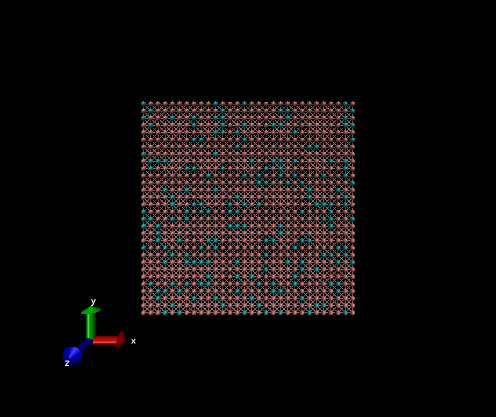
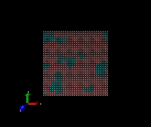
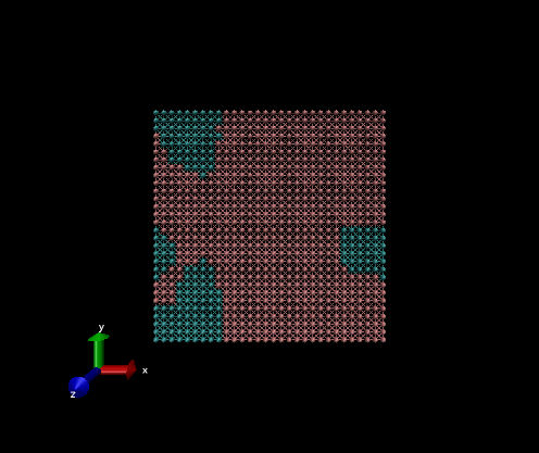
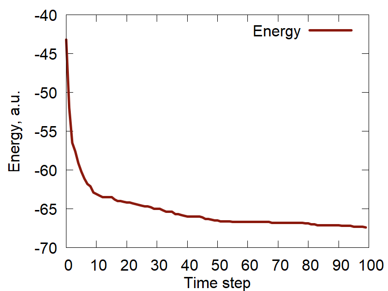
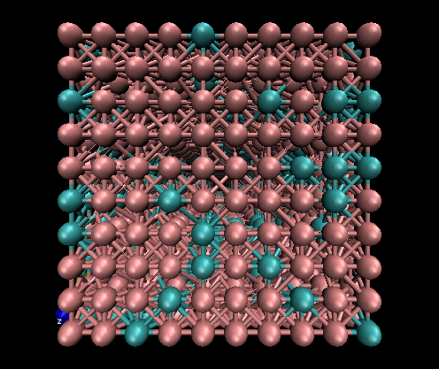
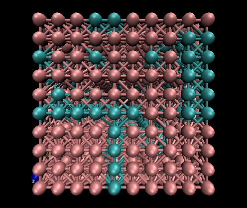
2D example

The variables that need be changed for this simulation are:

Nx, Ny, Nz = 20, 20, 1
pbc_opt = "ab"
nsteps = 500
f = open("2D/energy.txt", "w")
syst.print_ent("2D/step%i" % snap)  # two places
f = open("2D/energy.txt", "a")

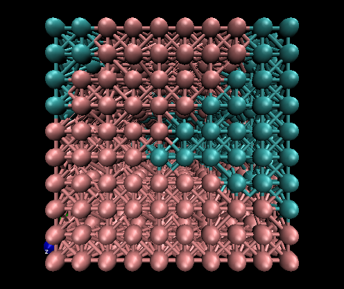
3D example

The variables that need be changed for this simulation are:

Nx, Ny, Nz = 10, 10, 10
pbc_opt = "abc"
nsteps = 100
f = open("3D/energy.txt", "w")
syst.print_ent("3D/step%i" % snap)  # two places
f = open("3D/energy.txt", "a")