Metropolis Monte Carlo Sampling
This tutorial shows how to utilize the Metropolis algorithm to sample data points from an arbitrary distribution defined by the user via Python script.
The working files can be found: hereTheory and implementation
The method is implemented in
the montecarlo library.
In Particular, we will be using the metropolis_gau function, which implements the Metropolis scheme with the
Gaussian random walk. The function accepts a multidimensional coordinate (of the MATRIX type), `q`, that defines the probability
distribution function, `P(q)`. The Metropolis sampling algorithm starts with some guess point of the variable `q(n=0) = q_0`. The
point `q_0` does not have to be included in the final sampling.
Then the following sequence of actions is executed repeatedly:
- A random vector, `xi = (xi_0, xi_1, ... , xi_N)`, is generated such that each of its component is sampled from the Gaussian distribution with the mean of 0.0 and variance of 1.0, `xi_i in G(0.0, 1.0)`. This vector is scaled by the desired variance magnitude, `sigma`, to define a proposed displacement vector, `sigma * xi`.
- A trial point is computed by displacing the vector, `q(n)`, by the amount of the proposed displacement vector: `q_{trial}(n+1) = q(n) + sigma * xi`
- The probability density defined by the user (the one, from which the points are being sampled) is evaluated at the new point: `P_{n ew} = P(q_{trial}(n+1))` and is compared to the present (to be old) probability density `P_{old} = P(q(n))`.
- If the instantaneous acceptance ratio is computed `a c c = (P_{n ew}) / P_{old}` is larger than 1.0, the proposed move is accepted with `100%` probability. Otherwise, the move is accpeted with the probability given by the `a c c`. The accepted moves update the coordinate, `q(n+1) = q_{trial}(n+1)`. The rejected moves do not change the coordinate, `q(n+1) = q(n)`. If the move is rejected, no new configuration is added to the results list.
In order to remove the potential dependence of the sampling on the starting point, the inital `Ns` = start_sampling points in the above sequence (we can even call it a trajectory) may be discarded. The resulting array of points `q(Ns), q(Ns+1), q(Ns+2), ..., q(Ss-1)` constitutes the returned result - the points sampled from the user-defined distribution.
One should be careful to choose the parameters of the metropolis_gau such that the best distribution is achieved
with minimal computational efforts. In particular: starting away from the maximum of the distribution, with the need for transitioninig
over the regions with low probability density may require prolonged simulation times (large sampling and large starting point),
now discarding enough initial points (especially if the total sampling size is small) may deteriorate the quality of the sample (non-
equilibrium effect), using very small Gaussian variance (step size) may slow down the convergence of sampling procedure. On the contrary,
using very large step size may lead to inaccurate sampling.
Below, we will consider several examples (motivated by the quantum mechanics course) of generating samplings drawn from complicated distributions. We will illustrate how the choice of the parameters affect the quality of the sampling.
The general scheme of the implementation of the sampling algorithm is demonstrated in Figure 1. The idea of the approach is to hide unnecessary details of the Metropolis algorithm implementation from the user, but yet allow the user to define an input function. Both the definition of the sampling distribution function and the call of the metropolis algorithm (together with the definition of other control variables) is performed at the Python level, easily accessible to the user. The computationally- intensive details of the algorithm are hidden in the C++ implemntation. The C++ function is also exposed to the Python level in order to be used by the user.
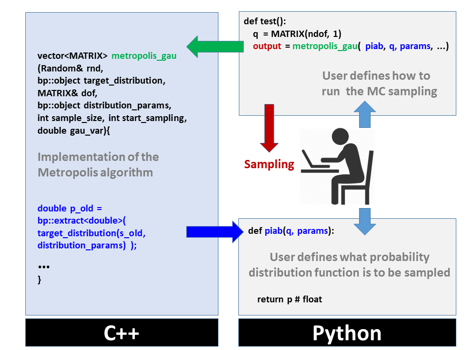 Figure 1.The schematic showing the oranization of the computations with the user-defined (in Python)
probability distribution function passed as an argument of the
Figure 1.The schematic showing the oranization of the computations with the user-defined (in Python)
probability distribution function passed as an argument of the metropolis_gau function.
Examples 1: Particle in a 1D box
The probability distribution function for a 1D particle in a box is defined by `P_n(x) = (2/L) sin^2({pi n x} / L)`.
In particular, we are interested in the test_piab.py file. The plot_piab.plt file can be used to generate the plots of the computed distributions.
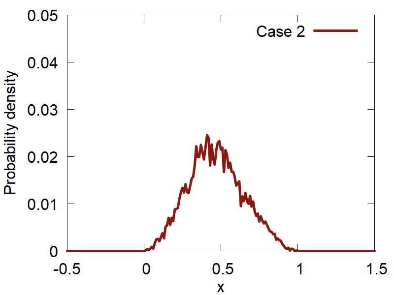
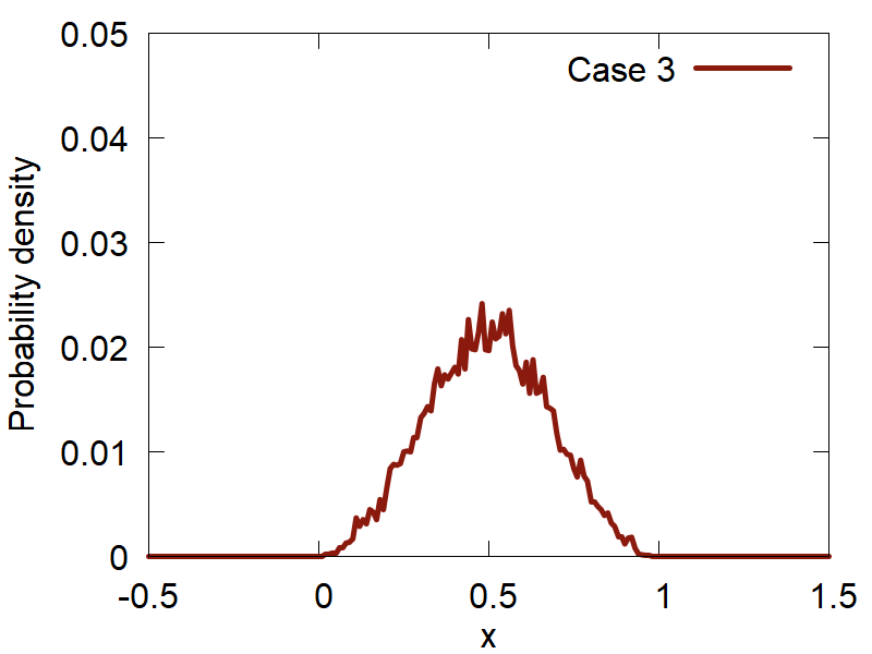
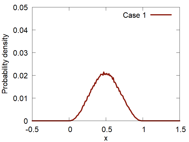
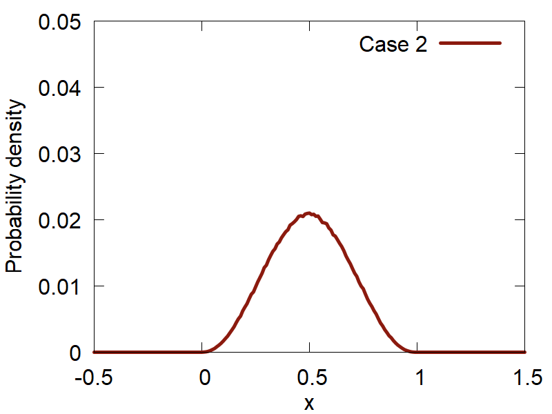
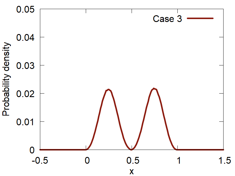
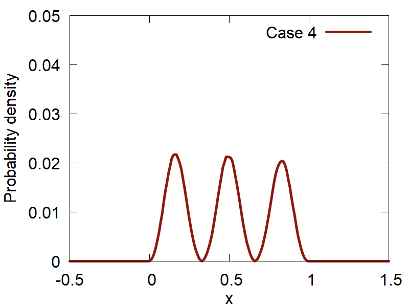
First, lets consider how the variation of the input parameters affects the quality of the computed distributions. The results are summarized in Figure 2:
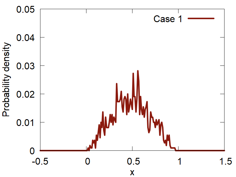
a
b
c

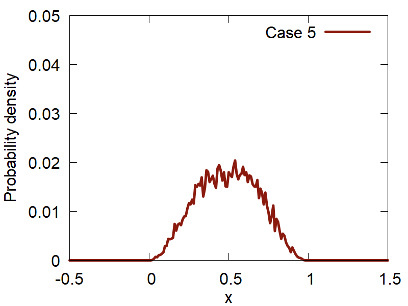
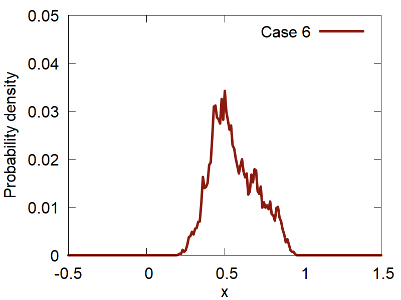
d
e
f
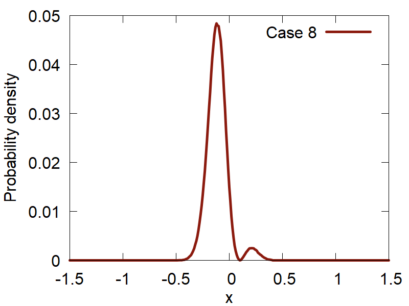
One can clearly observe how the version (d) (Case 4) shows the best distribution of all the tested ones. Please, take a look at how the variation of parameters changes the computed distributions and make your conclusions.
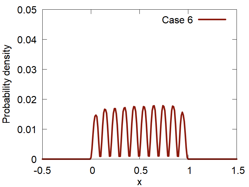
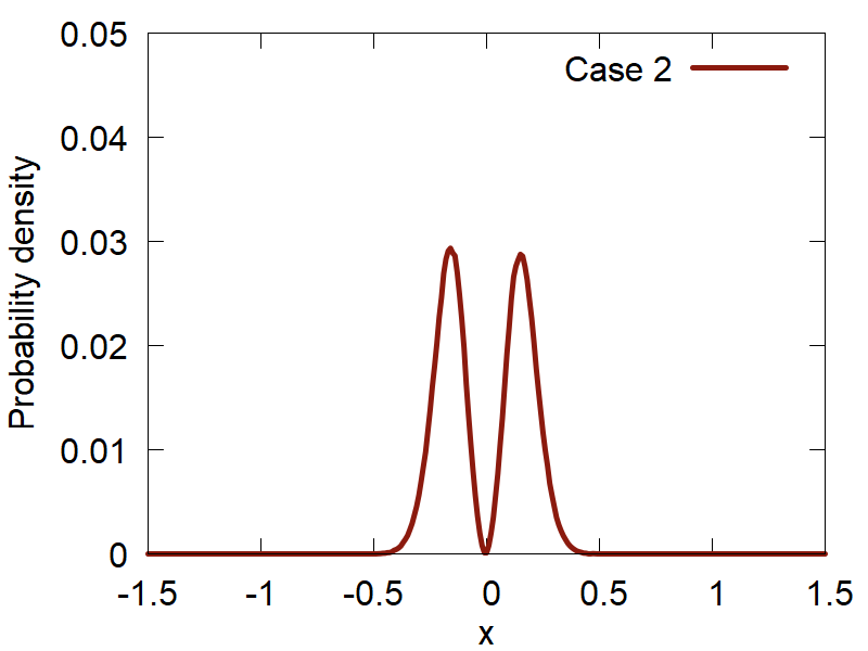
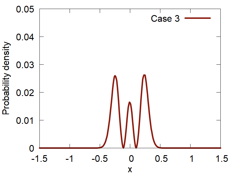
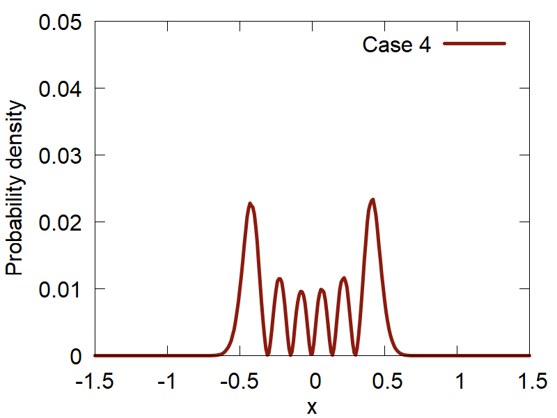
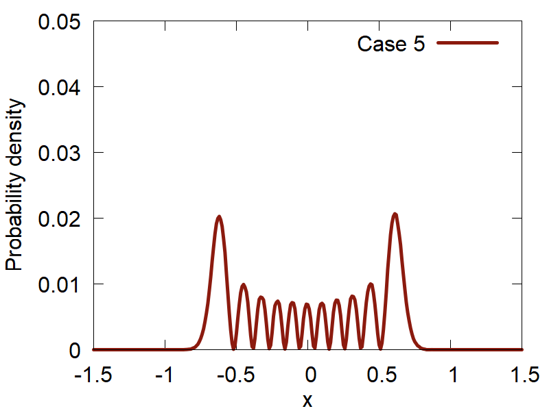
We can now go further and compute the distributions `P_n(x) = (2/L) sin^2({pi n x} / L)` for various n values, as
implemented in the function test_2 of the same module. The results are shown in Figure 3.
a
b
c

d
e
f
Examples 2: Probability Density of Harmonic Oscillator Superposition
In this exercise, we will consider sample points from the distributions that are given by the `|Psi(q,t)|^2`, where `Psi(q,t)` is a user-defined superposition of the Harmonic Oscillator (HO) eigenstates: `Psi(q,t) = sum_n{ c_n * |n(q) \> * exp(-{i E_n t} / {\hbar} ) }`. The HO eigenstates are given by: `|n(q) \> = N_n * H_n (q * \sqrt(alpha)) * exp(- {alpha q^2} / 2)`. Here, `H_n(x)` is a Hermite polynomial, `N_n = 1/\sqrt(2^n * n!) (alpha/pi)^(1/4)` is the normalization coefficient. The coefficient `alpha` is defined as `alpha = {m omega} / {\hbar}`, where `omega = \sqrt(k/m)`. Here, `k` is the harmonic force constant and `m` is the mass of the particle. The HO Hamiltonian to which this solution corresponds is `\hat H = \hat p^2 / {2 m} + k/2 * q^2`.
This tutorial is implemented in the test_ho.py file in the tutorial directory. The plot_piab.plt file can be used to generate the plots of the computed distributions.
Lets start with a simple case: `t = 0` and the superposition coefficients `c_n` are the constants given by the user. The points sampled from a number of superositions are shown in Figure 4.
a
b
c

d
e
f


g
h
i