Libmmath Tutorials
The "libmmath" module implements the basic mathematical functionality (in the object oriented way). The working files showing how to use different objects are located in the /tests/test_mmath directory of the Libra package. Most of the tutorials are almost completely self-explanatory. Here, we only focus on most interesting/less straightforward conventions and articulate some of our actions.
test_vector.py
We can create a VECTOR object by using a default constructor.
v1 = VECTOR()The vector stores 3 floating point numbers - x, y, and z coordinates. The default constructor sets all coordinates of v1 to zero.
The coordinates can be accessed via the members .x, .y, .z:
print v.x, v.y, v.zNote that the call
print vwould print the address of the object - this is useful to check the identity of that object, as will be discussed later.
The constructor can also take 3 arguments, to initialize all coordinates:
v2 = VECTOR(1.0, -2.0, 3.0)Another vector can be used to initialize a new vector.
v3 = VECTOR(v2)One can print the addresses of the vectors v2 and v3 to see that they are different. This means, that one can modify one object without affecting the other one.
Care must be exercised when dealing with assignments. In Python, all assignments are done by reference. This means that the assignent
v3 = v1would copy only the references. The variable v3 will then contain the reference to the previously created object v1. The main consequence of this is that the two "objects" are not independent. This is demonstrated in our tutorial. After the above assignent, we modify v1 and print both v1 and v3. You can see, that v3 now returns the same values as v1 - this is because v3 is merely a reference to the object v1. Analogously, one could affect v1 via modifying v3. By the way, this tricky side is common for all Python objects and complex data types, not only for Libra-spacific objects.
The trick doesn't work for the pair v2 and v3. This is because we called a constructor to create v3 from v2. The constructor allocates new memory and creates a totally independent object. To be on the safe side, call constructors (create new instances from scratch) whenever possible.
Next, the script demonstrates the arithmetic operations overloaded for the objects of the VECTOR class - addition, subtraction, multiplication and division by the real number are all defined:
v3 = v1 + v2
v3 = v1 - v2
v3 = 2.0*v1 - v2*3.0
v3 = v1/2.0
In addition, one can add up the vector and the number, which means the number will be added to all components of the new vector:
v3 = v1 + 1.0
Some build-in functions-members of VECTOR class are demonstrated: length and its square,
v1.length()
v2.length2()
normalizaition - affects the initial vector to make it bigger or smaller (such that eventually its length is 1.0):
v1.normalize()unit - returns the unit vector (a new object), but doesn't affect the original object:
v2 = v1.unit()cross - computes the cross-product (vector product) of the two vectors v1 and v2 and puts it in the vector v3:
v3.cross(v1,v2)the multiplication is overloaded such that the product of two vectors is essentially a scalar product:
x = v1*v2
Finally, we also demonstrate a very convenient feature - the vectorization of new data types. In order to be able to work with vectors
of custom classes, such as VECTOR, we have defined a set of *List classes, where * indicates the name of the class which we want to vectorize.
Specifically, the VECTORList class represents a list of objects, each of each is of VECTOR type. The object of such type corresponds to
C++ vectorvlst = VECTORList()
vlst = [v1, v2, v3]
print vlst[0] # this returns the address of the first vector
print vlst[1].x # this returns x component of the second vector in the list
test_matrix.py
To create a matrix of an arbitrary size containing real-valued elements we use:
a = MATRIX(3,3)To set the value of i-th row and j-th column to the value v, we use the "set" member-function:
a.set(i,j,v)To return the value in i-th row and j-th column, we use the "get" member-function:
print a.get(i,j)To print matrix out, we use the "show_matrix" member-function:
a.show_matrix
The description of more of MATRIX functionality will be added here later. So far, we can tell that, similar to VECTOR, many standard operations with objects of MATRIX and other types are overloaded to be most intuitive and follow standard mathematical conventions.
Among more advanced member-functions implemented in the MATRIX module the script demonstrates the eigenvalue solver using the Jacobi rotation method (which works only for symmetric matrices).
a.JACOBY_EIGEN(eva, eve, 1e-10)This function computes eigendecomposition of the matrix "a", and stores the eigenvectors and eigenvalues in the matrices "eve" and "eva", respectively. The number controls the desited accuracy. We further demonstrate the matrix multiplication operation by showing the results of the left- and right-hand sides of the eigenvalue problem: a * EVEC = EVEC * EVAL
(a*eve).show_matrix()
(eve*eva).show_matrix()
Finally, we demonstrate the performance of the JACOBY_EIGEN function, but applying it to matrices of increasing size. On my Cygwin/Windows system, the diagonalization of the biggest matrix 150 x 150 (which is pretty small) takes about 8 seconds (which is pretty slow). Thus, the algorithms may be suitable for small matrices. For larger matrices, one should use Eigen 3 functions wrapped in the "libmeigen" module (see the test_ceigen.py example). In this example, we also use the objects of the "Timer" class (see the test_timer.py) that is very convenient for the benchmark purposes.
test_matrix2.py
This script shows how to generate a sub-matrix from a bigger matrix (matrix popping) and how to populate a bigger matrix with the matrix elements of a smaller one (matrix pushing)
We first create a 5 x 5 matrix A:
N = 5
A = MATRIX(N,N)
We then populate the matrix with some numbers using the set() function:
A.set(i,j,-3*i+j*j)Printing of the generated matrix gives:
A.show_matrix()
>>>
              0              1              4              9             16
             -2             -1              2              7             14
             -4             -3              0              5             12
             -6             -5             -2              3             10
             -8             -7             -4              1              8
Lets also define another 5x5 matrix, B, with all elements set to zero. So, initially:
B.show_matrix()
>>>
              0              0              0              0              0
              0              0              0              0              0
              0              0              0              0              0
              0              0              0              0              0
              0              0              0              0              0
Now, lets say we want to extract a 2x2 matrix, a2x2, from the matrix A. First, we need to allocate memory by creating the actual object:
a2x2 = MATRIX(2,2)Next, we need to define which elements of the original matrix A we need to extract. This is done using the stensil - the list of the indices numerating colomns and rows the intersections of which will be extracted. For instance, if we want to get the upper left 2x2 block of the original matrix, we need to define the stensil as [0,1]. If we need the lower left 2x2 block, then we use [3,4]. Of course we can do something more interesting - lets say the elements on the intersections of the 2-nd and 4-th coloumns and rows - then we use the[1,3] stencil. So the results will be:
pop_submatrix(A,a2x2,[0,1]); a2x2.show_matrix();
>>>
              0              1
             -2             -1

pop_submatrix(A,a2x2,[3,4]); a2x2.show_matrix();
>>>
              3             10
              1              8

pop_submatrix(A,a2x2,[1,3]); a2x2.show_matrix();
>>>
             -1              7
             -5              3
We can now push the (last) extracted matrix a2x2 to the bigger matrix B:
push_submatrix(B,a2x2,[0,1]); B.show_matrix();
>>>
             -1              7              0              0              0
             -5              3              0              0              0
              0              0              0              0              0
              0              0              0              0              0
              0              0              0              0              0
To show more pushing lets use another matrix a3x3 and push it together with the matrix a2x2 into B. After resetting matrix B to zero and
extraxting ax3x3 from A in a certain way, lets do:
pop_submatrix(A,a3x3,[0,1,2]); B.show_matrix();
>>>
              0              1              4
             -2             -1              2
             -4             -3              0

push_submatrix(B,a3x3,[0,1,4]); B.show_matrix();
>>>
              0              0              0              1              4
             -0              0              0              0              0
              0              0              0              0              0
             -2              0              0             -1              2
             -4              0              0             -3              0
Important: the size of the stencil should be consistent with the size of the pushed/popped matrix
Potential use: for density matrix initialization - SAD - superposition of atomic densities. In addition, this technique can also be used for the fragmentation approaches - when you compute the density matrix for each fragment (in its own atomic basis - this is one of the submatrices) and then need to stitch the matrices together to produce the overall density matrix - in the space of all atomic orbitals.
test_ceigen
This script simply shows how to solve the (generalized) eigenvalue problem: H*C = S*C*E
We first generate the input matrices: the Hamiltonian matrix H is set to be real symmetric (hence Hermitian), the overlap matrix S is set to something other than trivial unity matrix:
H.show_matrix()
>>>
         -0.001          0.001
          0.001          0.001
S.show_matrix()

>>>
1.0000000      0.50000000
0.50000000     1.0000000
The eigenvalues and eigenvectors are then computed by a simple function:
solve_eigen(2, H, S, E, C)Note, that the eigenvectors and eigenvalues can, in general, be complex-valued. This is why we initialize matrices C and E as the CMATRIX objects:
E = CMATRIX(2,2)
C = CMATRIX(2,2)
To test the correctness of the eigenvalue solution, we compute the left- and right-hand sides of the equation H*C = S*C*E. However, since the multiplication of the complex and real matrices are is not defined yet, we need to convert the real matrices H and S into the complex counterparts (with zero imaginary components). This can be done using one of the overloaded constructors:
cH = CMATRIX(H); cH.show_matrix()
>>>
(-0.0010000000,0.0000000)  (0.0010000000,0.0000000)
(0.0010000000,0.0000000)  (0.0010000000,0.0000000)
cS = CMATRIX(S); cS.show_matrix()

>>>
(1.0000000,0.0000000)  (0.50000000,0.0000000)
(0.50000000,0.0000000)  (1.0000000,0.0000000)
How, we can test the solution:
(cH*C).show_matrix()
>>>
(0.0018739952,0.0000000)  (-0.00069867167,0.0000000)
(-0.00040337828,0.0000000)  (-0.0010819516,0.0000000)

(cS*C*E).show_matrix()
>>>
(0.0018739952,0.0000000)  (-0.00069867167,0.0000000)
(-0.00040337828,0.0000000)  (-0.0010819516,0.0000000)
We can also check the generalized orthogonality condition: C.H() * S * C = I
(C.H() * cS * C).show_matrix()
>>>
(1.0000000,0.0000000)  (-1.6653345e-16,0.0000000)
(-2.2204460e-16,0.0000000)  (1.0000000,0.0000000)
test_timer
This small test shows how to use the Timer object for measuring the computation times
To create the timer object we do:t = Timer()This is the only time the accumulator is set to zero. The accumulator contains the total time for all measured executions. The measurements are performed by setting the start point using
t.start()and the end point using
t.stop()When the stop function is called, the time between stop() and previous start() is measured and added to the accumulator. To show the total accumulated time, use the show() function
t.show()Since the only time the accumulator is set to zero is when the Timer object is created, there are two main usage modes of the Timer.
Mode A: Total time as in the first example:
t = Timer()
for a in xrange(3):
    t.start()
	... here goes the task the time of which we measure ...
    t.stop()
    print "Time to compute = ", t.show(), " sec"
In this mode, we create the Timer object only once, and then store the total time for each cycle of computations
Mode B: Time per iteration as in the second example:
for a in xrange(3):
    t = Timer()
    t.start()
    ... here goes the task the time of which we measure ...
    t.stop()
    print "Time to compute = ", t.show(), " sec"
In this more we create the Timer object for each cycle, and hence the time returned by the show() function corresponds to the time needed
for each single computational cycle.
Random numbers generator: test.py
This example shows how to generate some relatively standard random distributions: uniform (well, this is nothing but a wrapper of the intrinsic C++ functions), exponential, normal, and some other. The example also shows how to analyze the randomly distributed numbers, to plot some distributions.
The very first step needed to generate random numbers in Libra, is to create an object of the Random class. This object is a container of the pseudorandom number sequences. This object has a common random seed, set up at the time of the object creation. Therefore, the object must be created only once and then appropriate random numbers can be extracted from the sequence. If new instance of the object is created every time the random number is extracted, the sequence of the obtained numbers will contain many repetition of the same numbers, unless the time between each call is large enough to obtain (system clock-dependent) very different random seed. The principle is illustrated by running a small loop generating 10 random numbers (Test 1 and Test 1a). The particular number you'll see in the Test1 will vary each time you run the code, but it will stay more or less the same for all iterations. For instance:
Test 1: Constructor is called each time when the number is generated
0 0.26743836434
1 0.26743836434
2 0.26743836434
3 0.26743836434
4 0.26743836434
5 0.26743836434
6 0.26743836434
7 0.26743836434
8 0.26743836434
9 0.26743836434

Test 1a: Constructor is created only once
0 0.26743836434
1 0.761646950041
2 0.584602647733
3 0.541262961245
4 0.0468970956499
5 0.420079873605
6 0.808454720214
7 0.564376205469
8 0.633402130396
9 0.384234171074
To analyze the generated random numbers, we utilize the DATA class. The constructor takes a list of random numbers to store them internally:
dy1 = DATA(y1)
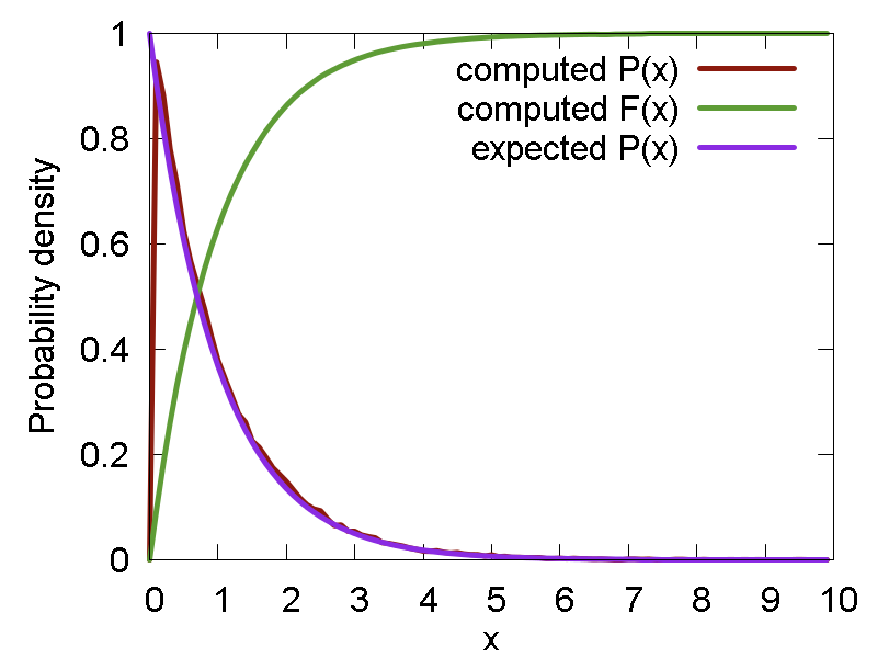
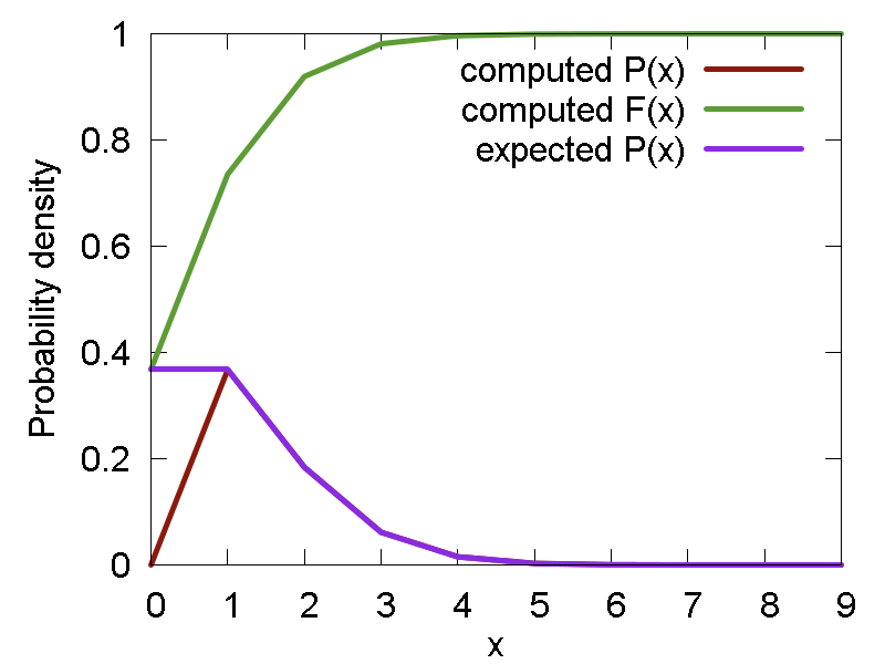
To compute the density function for the sampled random numbers, we utilize the "Calculate_Distribution" method of the DATA class. The function takes another list, the one that defined the grid points (support of the distribution) and returns a list of two lists: The very first element of the returned list is a probability density function for all grid points (a list), `P(x)`. The second element of the returned list is a cumulant function: `F(x) = int_(-oo)^x P(x)dx` - the density function integrated up to the given grid point:
dens, cum = dy1.Calculate_Distribution(x)
To generate different random distribution, we call the appropriate functions (members of the class Random). The available distributions are:
- Uniform distribution: `P(x; a, b) = 1/(b-a)`. Methods: "uniform" - generates the numbers, "p_uniform" - computes the corresponding probability density function
- Exponential distribution: `P(x; lambda) = lambda * e^(-lambda * x)`. Methods: "exponential" - generates the numbers, "p_exponential" - computes the corresponding probability density function
- Normal distribution: `P(x) = (2 pi)^(-1/2) * e^(- 1/2*x^2)`. Methods: "normal" - generates the numbers, "p_normal" - computes the corresponding probability density function
- Poisson distribution: `P(n; lambda) = e^(-lambda)*lambda^n/(n!)`. Methods: "poiss1", "poiss2" (both correspond to n = 1) - generate the numbers, "p_poiss" - computes the corresponding probability density function
- Gamma and beta distributions are also available, but need more testing and description
Examples of the random numbers generated and the related distribution functions (density and cumulant) are shown below:
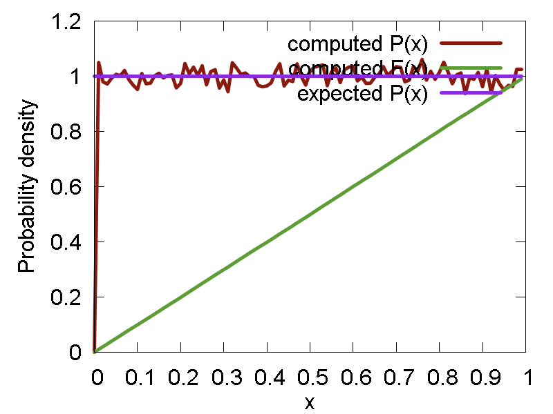

a
b

c
d
e
Metropolis algorithm: test2.py
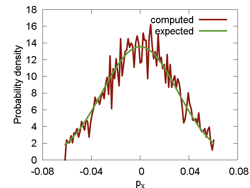
Sometimes, we need to sample random numbers from a significantly more complex distributions. In this cases, the Metropolis sampling algorithm is a standard choice, especially in physical chemistry problems. In the present example we implement a Metropolis algorithm for sampling phase space points (both coordinates, `x`, and the momenta, `p_x`) from the Boltzmann distribution, `P(q,p) = 1/Z*exp(-(H(q,p))/(k_B T))`,corresponding to a given Hamiltonian, H(q,p). Here, `Z` is the partition function. In particular, we use a simple Harmonic oscillator Hamiltonian: `H(q, p) = p^2 /2 + 1/2*omega^2*x^2 + M*x`, where `M = (1/2*omega^2 * E_r)^(1/2)` This is implemented in the
boltz()function defined in the beginning of the script. What the function does, is essentialy a random walk in the 2-dimensional phase space. Along the walk, new configurations are proposed and then either accepted or regected according to the Metropolis algorithm. After sufficiently long run (1000 steps, in this example) the generated point is assumet to a statistically-independent one, drawn from the proper distribution. It is then returned upon the call of the "boltz" function.
We generate 5000 pairs of numbers `(q, p)` and then compute probability distribution functions alsong q and p axes. The computed distributions are compared with the Boltzmann populations computed numerically for the given 2D grid. The results are presented in Figure 2.

a
b
Pseudorandom numbers generation: test3.py
Well, this is not an intrinsic functionality of Libra, but rather just an interesting test case. One of the ineresting ways of generating "random" (really, pseudo-random) numbers is via deterministic mapping with the parameters chosen such that the mapping enters a chaotic regime. In particular, we consider the mapping `x_(n+1) = 4*r*x_n*(1-x_n)`, where `0 < r < 1` is a parameter. Depending on the choice of `r`, the mapping may enter a chaotic regime and would generate a sequence of pseudorandom numbers. The
Calculate_Distribution(x)is useful here to analyze the probability density of the generated numbers.
For instance, we use the parameters `r = 0.98` and `x_0 = 0.2`. The generated sequence, as well as the corresponding density and cumulant functions are shown in Figure 3.


a
b